![]()
Aqueduct Fluidics makes automation more accessible for benchtop-scale applications in research and development and in small scale production.
Our platform empowers users to conceive, design, simulate, and deploy complex systems with confidence.
The platform simplifies system integration by handling challenging elements such as communication and command timing, user interfaces, and data persistence. Users can focus on their specific protocols while the platform takes care of the underlying complexities.
Key Benefits:
-
Simple, Flexible Scripting
Aqueduct Recipes are written in Python (3.7+), the widely adopted scripting language. Leveraging the power of Python's standard library and the Aqueduct API, users can easily program processes without sacrificing the flexibility required for their specific applications.
-
Built-In System and Data Visualization
The Aqueduct interface provides an intuitive and flexible environment for controlling and visualizing the status of your hardware. It features an icon-based representation of the hardware, live plotting and graphing utilities, and programmable user interactions. The interface can be customized to suit individual preferences and application requirements.
-
Simulation of Processes without Hardware
The Aqueduct platform offers simulation-only representations of each type of hardware component. These emulated devices faithfully mimic the behavior of real hardware, allowing users to develop and test Recipes without the need for physical lab equipment. Additionally, users can simulate noise or time-dependency in signals to accurately model their processes and control algorithms.
-
Ecosystem of Application Use Cases and Code Blocks for Rapid Development
Our platform provides an ecosystem of pre-existing, application-specific Libraries and Recipes that can be utilized off-the-shelf or customized to suit individual needs. Alternatively, users can leverage our collection of code snippets and templates to build their solutions from scratch, minimizing development time.
![]()
Tangential Flow Filtration (TFF) - also referred to as cross flow filtration - is a fast and effective technique for separating and purifying biomolecules.
In the TFF process, fluid flows tangentially along the surface of a filter membrane. Through the application of a pressure differential within the system, smaller constituents that can pass through the membrane's pore structure are directed into the filtrate, while larger constituents are retained and recirculated along the system's flow path.
TFF is utilized across diverse biological domains including immunology, protein chemistry, molecular biology, biochemistry, and microbiology. TFF is effective for concentrating and desalting sample solutions, fractionating large and small biomolecules, collecting cell suspensions, and clarifying fermentation broths and cell lysates.

Control is Paramount
Control is paramount in TFF. Precise manipulation of key parameters drives the efficiency and effectiveness of the process. Key control parameters include:
Transmembrane Pressure (TMP)
Transmembrane pressure -- the differential pressure across the filter membrane -- plays a pivotal role in process efficiency. By controlling the pressure differential across the membrane, the permeation of substances through the filter can be precisely managed, ensuring the desired separation and purification outcomes.

Crossflow Rate
In conjunction with the TMP, crossflow rate plays a significant part in determining process yield. By optimizing the crossflow rate, fouling and clogging risks are minimized, leading to consistent and reliable results.

Feed Concentration
In continuous diafiltration, salts or solvents (low molecular weight species) in the feed liquid are continuously removed by passes through the filter cartridge. As the unwanted species are pulled through the filter membrane, a replacement buffer (or water) solution is added to the feed container to keep the concentration constant.

Control over these parameters isn't just about achieving optimal results; it's about reproducibility and scalability. A well-controlled TFF process ensures that results obtained in the laboratory can be translated to larger-scale applications with confidence.
The Aqueduct Fluidics openTFF System
We're building the Aqueduct Fluidics openTFF system to be a comprehensive automation solution tailored for lab-scale TFF processes.
The system includes an embedded computer and a dedicated interface board, both enclosed in a sealed housing.
The interface board features three dedicated Mixed IO (MIO) interfaces designed to control laboratory pumps (see a list of compatible pumps here). A 4-20mA speed control output signal and a 4-20mA tachometer input signal enable low-latency speed control and real-time volume accumulation for accurate volume measurement and precise finite dispenses. Two isolated digital outputs enable the manipulation of run and direction toggles while an isolated digital input provides monitoring of pump status (running or stopped).
Four serial communication ports facilitate communication and control of a range of peripherals such as balances, pressure transducers, and recirculating baths, enhancing the system's flexibility and applicability across various setups. By simply configuring the application to recognize the peripheral you have connected, the Aqueduct drivers take care of reading data into the application.
The system includes an Aqueduct Comm bus. This 4-wire, full-duplex RS485 communication interface is exclusively dedicated to interfacing with the Aqueduct pinch valve or other additional nodes, thereby offering the potential for system expansion and integration with other components.
Built for Flexibility
The system's modular design allows you to tailor your setup according to your specific process needs. The system allows you to integrate a variety of components, including balances, pH probes, conductivity probes, pressure transducers, and recirculating baths.
Scalability and Adaptability
The openTFF system is designed to grow with your requirements. As your process evolves, you can expand the system by adding new components or functionalities. This scalability ensures that your investment remains relevant and valuable over time, accommodating changing demands and advancing technologies.
Integration with Existing Setup
The openTFF system may be compatible with your existing equipment. Whether you already have certain pumps, sensors, or instruments in place, the system's adaptability enables it to seamlessly integrate with your current laboratory infrastructure.
Full Utilization of Aqueduct Capabilities
By leveraging the capabilities of the Aqueduct platform, the openTFF system provides advanced features that enhance your TFF processes:
-
Simulation Mode: Test and refine your process logic in a simulated environment, minimizing risks and optimizing parameters before implementing them in the actual setup.
-
Event Logging: Capture real-time data and events for comprehensive process documentation, analysis, and troubleshooting. This valuable information supports quality control and process improvement efforts.
-
Third-Party Integration: Integrate third-party databases or APIs into the Aqueduct platform, enabling enhanced data management. This integration expands the system's potential applications and connectivity.
Streamlined Process Development
The openTFF system accelerates process development by offering a user-friendly interface for configuring and controlling various components. The ability to fine-tune parameters and visualize their impact allows for rapid optimization and quicker process deployment.
Contact Us
If you're interested in learning more about the system or have specific requests for peripherals you would like to see added, contact us at info@aqueductfluidics.com.
Interface Circuit Board
The openTFF Interface board includes three specialized Mixed I/O (MIO) interfaces tailored for pump control, four configurable serial communication ports, and an Aqueduct CommBus interface. These interfaces ensure precise control, data communication, and expansion possibilities.

Three Dedicated Mixed I/O Ports for Controlling Pumps
The openTFF system is equipped with three specialized Mixed I/O (MIO) interfaces designed to control pumps (peristaltic, piston, and diaphragm) commonly used in a TFF setup. These MIO interfaces feature:
-
4-20 mA Speed Control Channel: This channel transmits a 4-20 mA signal used to control the speed of a pump, ensuring accurate and precise fluid flow rates.
-
4-20 mA Tachometer Input Channel: The tachometer input channel is responsible for receiving a 4-20 mA signal from the pump's tachometer. The tachometer measures the rotational speed (or a proxy for flow rate, depending on the model) of a pump. The interface not only monitors the pump's speed but also accumulates real-time data to calculate the total volume of fluid displaced, enabling finite dispense operation.
-
Digital Inputs and Outputs Channels: Two digital output channels and a digital input channel are used to control the run and direction toggles of the connected pump and monitor the pump's status.
8 pin M12 A-code plug, male pins

|
|
Four Configurable Serial Interfaces
In addition to the three specialized MIO interfaces, the openTFF system includes four serial communication ports. In conjunction with the Aqueduct software, these ports can be configured to interface with various peripherals commonly used in TFF setups. Among these ports, two can be configured for half-duplex RS485 communication, enhancing compatibility with a wide range of industrial devices.
3 pin M8 A-code plug, male pins

|
|
Aqueduct CommBus Interface
8 pin M12 A-code receptacle, female pins

|
|
Supported Hardware (Preliminary)
Balances
| Brand | Supported Models | Interface Type | External Node Required | Connections |
|---|---|---|---|---|
| Mettler Toledo | XP/XS Series, XPE/XSE Series | RS232 | no | (coming soon) |
| Sartorius | Cubis, Quintix | RS232 | no | (coming soon) |
| Ohaus | Explorer®, Adventurer®, Scout® Series | RS232 | no | link |
Pressure Transducers
| Brand | Supported Models | Interface Type | External Node Required | Connections |
|---|---|---|---|---|
| Parker SciLog® | SciPres® | RS232 | no | link |
| Pendotech | PressureMAT® | RS232 | no | (coming soon) |
pH Probes
| Brand | Supported Models | Interface Type | External Node Required | Connections |
|---|---|---|---|---|
| Aqueduct pH ADC Node | most standard pH electrodes (supports 3) | BNC | yes | (coming soon) |
| Thermo Fisher | Orion Star A Series | RS232 | no | (coming soon) |
Conductivity Probes
| Brand | Supported Models | Interface Type | Inline/Immersion | External Node Required | Connections |
|---|---|---|---|---|---|
| Parker SciLog® | SciCon® | RS232 | inline | no | (coming soon) |
| Thermo Fisher | Orion Star A Series | RS232 | no | (coming soon) |
Pinch Valves
| Brand | Supported Models | Interface Type | External Node Required | Connections |
|---|---|---|---|---|
| Aqueduct | Pinch Valve | Aqueduct CommBus | yes | link |
MIO Pumps
MIO Port - Masterflex L/S® DB25 Connections

|

|
| Aqueduct MIO Pin | Signal | Masterflex L/S® Female Receptacle DB25 Pin |
|---|---|---|
| 1 | Aux Ground | 13 |
| 2 | Aux +24V | 25 |
| 3 | 4-20 mA RX, Tachometer | 4 |
| 4 | 4-20 mA TX, Speed Control | 2 |
| 5 | Running Digital In | 6 |
| 6 | Run Digital Out | 15 |
| 7 | Direction Digital Out | 16 |
| 8 | Aux Ground | 3 |
Recommended Cable Assembly Bill of Materials
| Manufacturer | Part Description | Part Number | Quantity |
|---|---|---|---|
| Phoenix Contact | Sensor/actuator cable, 8-position | 1406105 | 1 |
| Cinch Connectivity | 25 Position Two Piece Backshell Connector | 40-9725HMG | 1 |
| TE Connectivity AMP Connectors | 25 Position D-Sub Plug, Male Pins | 5-747912-2 | 1 |
| Conductor Number | Conductor Color | D-Sub Plug DB25 Pin |
|---|---|---|
| 1 | White (⚪) | 13 |
| 2 | Brown (🟤) | 25 |
| 3 | Green (🟢) | 4 |
| 4 | Yellow (🟡) | 2 |
| 5 | Grey (⚪) | 6 |
| 6 | Pink (🟣) | 15 |
| 7 | Blue (🔵) | 16 |
| 8 | Red (🔴) | 3 |
Further information in the Masterflex L/S® manual here.
See instructions for configuring the pump and calibrating the speed control and tachometer output signals here.
MIO Port - Watson Marlow DB25 Connections
|
|

|
| Aqueduct MIO Pin | Signal | Watson Marlow 530U, 630U Upper Male Plug DB25 Pin |
|---|---|---|
| 1 | Aux Ground | 16 |
| 2 | Aux +24V | 20 |
| 5 | Running Digital In | 10 |
|
|
|
| Aqueduct MIO Pin | Signal | Watson Marlow 530U, 630U Lower Female Receptacle DB25 Pin |
|---|---|---|
| 3 | 4-20 mA RX, Tachometer | 12 |
| 4 | 4-20 mA TX, Speed Control | 4 |
| 6 | Run Digital Out | 7 |
| 7 | Direction Digital Out | 6 |
| 8 | Aux Ground | 14 |
Further information in the Watson Marlow 530U manual here.
Balances
Serial Port - Ohaus RS232 DB9 Connections

|

|
| Aqueduct Comm Pin | Signal | Ohaus RS232 Female Receptacle DB9 Pin |
|---|---|---|
| 1 | Ground | 5 |
| 3 | Rs485 A/Rs232 Tx | 3 |
| 4 | Rs485 B/Rs232 Rx | 2 |
Recommended Cable Assembly Bill of Materials
| Manufacturer | Part Description | Part Number | Quantity |
|---|---|---|---|
| Phoenix Contact | Sensor/actuator cable, 3-position | 1406318 | 1 |
| Cinch Connectivity | 9 Position Two Piece Backshell Connector | 40-9709HMG | 1 |
| TE Connectivity AMP Connectors | 9 Position D-Sub Plug, Male Pins | 5-747904-2 | 1 |
| Conductor Number | Conductor Color | D-Sub Plug DB9 Pin |
|---|---|---|
| 1 | Brown (🟤) | 5 |
| 3 | Blue (🔵) | 3 |
| 4 | Black (⚫) | 2 |
Further information in the Ohaus Scout RS232 interface manual here.
See instructions for configuring the balance here.
Pressure Transducers
Serial Port - Parker SciLog® SciPres® DB9 Connections
|
|
|
| Aqueduct Comm Pin | Signal | SciLog® SciPres® RS232 Female Receptacle DB9 Pin |
|---|---|---|
| 1 | Ground | 5 |
| 3 | Rs485 A/Rs232 Tx | 3 |
| 4 | Rs485 B/Rs232 Rx | 2 |
Recommended Cable Assembly Bill of Materials
| Manufacturer | Part Description | Part Number | Quantity |
|---|---|---|---|
| Phoenix Contact | Sensor/actuator cable, 3-position | 1406318 | 1 |
| Cinch Connectivity | 9 Position Two Piece Backshell Connector | 40-9709HMG | 1 |
| TE Connectivity AMP Connectors | 9 Position D-Sub Plug, Male Pins | 5-747904-2 | 1 |
| Conductor Number | Conductor Color | D-Sub Plug DB9 Pin |
|---|---|---|
| 1 | Brown (🟤) | 5 |
| 3 | Blue (🔵) | 3 |
| 4 | Black (⚫) | 2 |
Note: Connect to the Female DB9 port labelled "Printer/PC".
Further information in the Parker SciLog® SciPres® manual here.
See instructions for configuring the balance here.
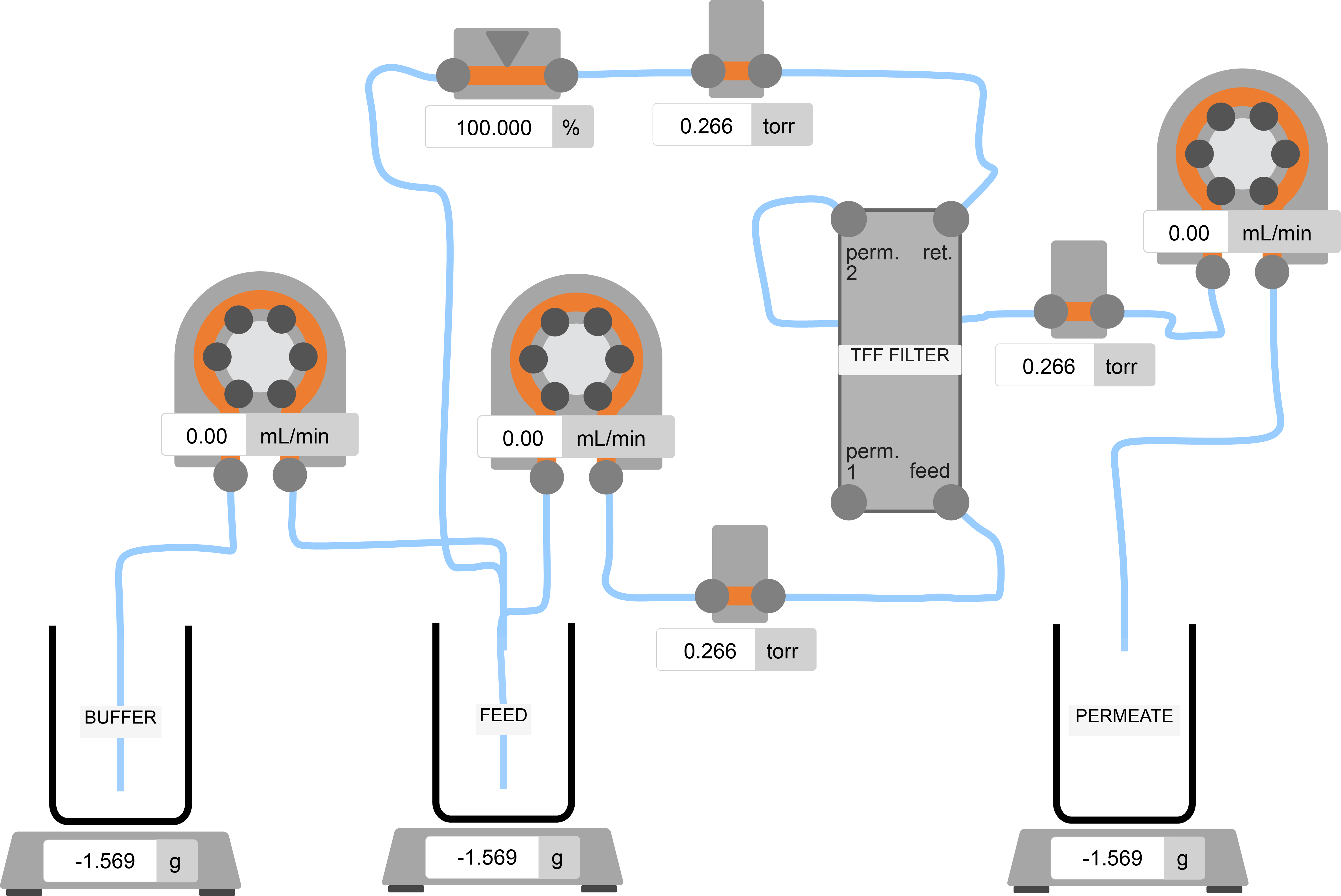
Simulating a TFF Process Using the Aqueduct Application
The Aqueduct application provides simulation capabilities that allow for the modeling of a TFF process. This guide outlines how to model the process using mathematical equations and Python code. It covers calculations for retentate, feed, and permeate pressures, as well as rates-of-change for balances that measure buffer, feed, and permeate product volumes.
The approach outlined in this guide is not limited to TFF systems; it can be readily adapted for other in-line and batch bioprocess applications.
- Process Variables
- Calculating Pinch Valve \( \text{Cv} \)
- Calculating Retentate Pressure
- Calculating Feed Pressure
- Calculating Permeate Pressure
- Calculating Balance Rates-of-Change
- Appendix
Independent Process Variables
The model takes the following independent variables as input parameters:
- Feed Pump Rate - Flow rate of the feed pump (e.g., mL/min).
- Buffer Pump Rate - Flow rate of the buffer pump (e.g., mL/min).
- Permeate Pump Rate - Flow rate of the permeate pump (e.g., mL/min).
- Pinch Valve Position - Position of the pinch valve, converted into a Valve Flow Coefficient (Cv) value.
The independent process variables are set by user interactions (either through the UI or a an Aqueduct Recipe).
Dependent Variables
Using the independent process variables, the simulation calculates the following dependent variables:
- Feed Pressure - Pressure at the feed side of the filter.
- Retentate Pressure - Pressure on the retentate side of the filter.
- Permeate Pressure - Pressure on the permeate side of the filter.
- Weight on Buffer Balance - Weight rate-of-change on the buffer balance.
- Weight on feed Balance - Weight rate-of-change on the feed balance.
- Weight on Permeate Balance - Weight rate-of-change on the permeate balance.
graph TD

A[Start] --> B[Calculate Pinch Valve Cv];
B --> C[Calculate Retentate Pressure<br>using Pinch Valve Cv and Feed Rate];
C --> D[Calculate Feed Pressure<br>using Permeate Pressure, Filter Cv, and Feed Rate];
D --> E[Calculate Permeate Pressure<br>using Feed and Retentate Pressure<br>and Permeate Flux];
E --> F[Calculate Mass Accumulation<br>on Feed, Buffer, and Permeate<br>Balances using Feed Rate,<br>Permeate Flux, and Buffer Pump Rate];
F --> G[End];

click B "#calculating-pinch-valve-textcv" _blank
click C "#calculating-retentate-pressure" _blank
click D "#calculating-feed-pressure" _blank
click E "#calculating-permeate-pressure" _blank
click F "#calculate-balance-rates-of-change" _blank
Calculating Pinch Valve \(\text{Cv}\)
We start the \(\text{Cv}\) calculation by estimating the percentage of occluded area in the cross-section of a tube based on its change in height (\( \Delta h \)).
The underlying mathematics are derived from this paper. The occlusion value scales between 0 and 1, where 1 indicates maximum occlusion (tube completely pinched), and 0 indicates no occlusion (tube retains original shape).
@staticmethod
def occluded_area_pct(delta_h: float) -> float:
    """
    Calculate the percentage change in cross-sectional area of a
    tube when it's squeezed, based on the change in height.

    See: https://www.hindawi.com/journals/mpe/2015/547492/

    Parameters:
    delta_h (float): The change in height due to the squeeze as a
    fraction of the original height (ranging from 0 to 1).

    Returns:
    float: The percentage change in the new cross-sectional area, scaled between 0 and 1.
        1 indicates maximum occlusion (tube completely flat),
        0 indicates no occlusion (tube retains original shape).
    """
    x = max(.5 - delta_h, 0)
    oc = math.pi * x * (math.sqrt(-20 * x**2 + 12 * x + 3) / 6 - (2 * x / 3) + 0.5)
    oc = min(-1 * (oc-0.7853981633974483), 1)
    return oc
The occluded area vs. \( \Delta h \) relationship is illustrated in the following plot:

After calculating the percentage of occluded area, we scale the original tube cross sectional area using the inner diameter in mm to \(\text{Cv}\) value using the functions:
@staticmethod
def cv_from_area_mm(area_mm: float) -> float:
    # Convert the area from mm^2 to m^2
    area_m = area_mm * 1e-6

    # Calculate the diameter from the area
    diameter_m = math.sqrt((4 * area_m) / math.pi)

    # Calculate Cv using the given formula
    Cv = (((diameter_m) ** 2) * 0.61) * 46250.9

    return Cv

@staticmethod
def calc_pv_cv(position: float) -> float:
    """
    Calculate the Cv of the pinch valve.

    :param PV: Pinch valve position.
    :type PV: float

    :return: Cv of the pinch valve.
    :rtype: float
    """
    response_zone = 0.35

    if position < response_zone:
        area = (math.pi * (5 / 2)**2)  * \
          (1 - PressureModel.occluded_area_pct((response_zone - position)/response_zone))
        return PressureModel.cv_from_area_mm(area_mm=area)
    else:
        return 100
Pinch Valve \(\text{Cv}\) Calculation
Next, we calculate the \(\text{Cv}\) value using the following steps:
-
Check Valve Position: If the valve's open position is below the
response_zonethreshold (0.35), we proceed to calculate the Cv by adjusting the cross-sectional area of the tube. This simulates the large range of the pinch valve position that does not have any affect on the tubing restriction area and will help us to develop control algorithms later. -
Calculate Occluded Area: We use the
occluded_area_pctmethod to find the percentage of the tube's area that is occluded or squeezed due to the valve's position. -
Scale Original Tube Area: The original cross-sectional area of the tube (calculated using the tube's inner diameter of 5 mm) is then scaled by
(1 - occluded_area_pct)to find the actual cross-sectional area when the valve is at the given position. -
Calculate Cv: With the actual area in hand, we proceed to calculate the Cv value using the
cv_from_area_mmmethod.
The following plot illustrates the relationship between \(\text{Cv}\) and the pinch valve position (in percent open, from 0 to 1).

Calculating Retentate Pressure
After we've calculated the flow coefficent \(\text{Cv}\) of the pinch valve based on its position, we can calculate the retentate pressure.
-
Obtain Feed Pump Rate: We use the (independent) feed pump rate process variable to set the mass flow through the restriction, \(Q\).
-
Apply Flow-Pinch Valve Relationship: The pressure drop across a restriction is related to the flow rate \(Q\) and the \(\text{Cv}\) of the restriction by the equation:
\[ \Delta P_{\text{psi}} = \left( \frac{Q}{0.865 \times \text{Cv}} \right)^2 \times 14.5038 \]
Here, \(\Delta P\) is the pressure drop across the valve, \(Q\) is the mass flow rate in \(\frac{m^3}{hr}\), and \(\text{Cv}\) is the flow coefficient of the restriction.
In Python, the calc_delta_p_psi method is used to perform the calculation:
@staticmethod
def calc_delta_p_psi(mass_flow_rate_ml_min: float, cv: float) -> float:
    """
    Calculate the pressure drop between through a restriction
    using the metric equivalent flow factor (Kv) equation:

    Kv = Q * sqrt(SG / ΔP)

    Where:
    Kv : Flow factor (m^3/h)
    Q : Flowrate (m^3/h)
    SG : Specific gravity of the fluid (for water = 1)
    ΔP : Differential pressure across the device (bar)

    Kv can be calculated from Cv (Flow Coefficient) using the equation:
    Kv = 0.865 * Cv

    :param mass_flow_rate_ml_min: Flowrate.
    :type mass_flow_rate_ml_min: float

    :param cv: Flow Coefficient.
    :type cv: float

    :return: Pressure drop (psi).
    :rtype: float
    """
    try:
        kv = 0.865 * cv
        # Convert mL/min to m^3/h
        delta_p_bar = 1 / (kv / (mass_flow_rate_ml_min / 60.0)) ** 2
        delta_p_psi = delta_p_bar * 14.5038  # Convert bar to psi
        return delta_p_psi
    except ZeroDivisionError:
        return 0
- Calculate Retentate Pressure: Now that we have \( \Delta P \), we can calculate the retentate pressure using the following equation:
\[ P_{\text{Retentate}} = P_{\text{atm}} + \Delta P \]
where \( P_{\text{atm}} \) is atmospheric pressure. \( \Delta P \) is the pressure drop across the pinch valve, which we calculated earlier. Since we're interested in gage pressure (pressure above atomospheric pressure), we can neglect \( P_{\text{atm}} \) and:
\[ P_{\text{Retentate}} = \Delta P \]
The relationship between feed rate (in mL/min), pinch valve position (from 0 to 1, 1 being fully open), and the retentate pressure is illustrated in the following plot:

Calculating Feed Pressure
Once we know the retentate pressure, we can calculate the feed pressure using the \(\text{Cv}\) value for the pass-through stream of the TFF filter and the mass flow rate, as set by the feed pump.
The \(\text{Cv}\) value represents the flow coefficient of the pass-through stream's filter section.
The equation for calculating the feed pressure \( (P_{\text{feed}}) \) is:
\[ P_{\text{feed}} = P_{\text{retentate}} + \Delta P_{\text{pass-through}} \]
Where \( \Delta P_{\text{pass-through}} \) is the pressure drop across the pass-through leg of the TFF filter. This pressure drop can be calculated using the calc_delta_p_psi() function, which takes in the mass flow rate and \(\text{Cv}\) value as parameters and returns \( \Delta P \) in psi.
Here is the relevant Python code snippet to compute \( P_{\text{feed}} \):
def calc_feed_pressure_psi(
    self,
    feed_rate_ml_min: float,
    retentate_pressure_psi: float
  ) -> float:
    """
    Calculate the feed pressure.

    :param feed_rate_ml_min: Flow rate in the pass-through leg of the TFF filter (ml/min).
    :type feed_rate_ml_min: float

    :param retentate_pressure_psi: Retentate pressure (psi).
    :type retentate_pressure_psi: float

    :return: feed pressure (psi).
    :rtype: float
    """
    return retentate_pressure_psi + \
      self.calc_delta_p_psi(feed_rate_ml_min, PressureModel.filter_cv_retentate)
Experimental measurements yield \(\text{Cv}_{filter} \approx 0.86\) for our Pelicon filter.
Calculating Permeate Pressure
Once we have the retentate and feed pressures, we can calculate the permeate pressure.
The formula for calculating the permeate pressure is based on the work by Juang et al., who used a resistance-in-series model to estimate the permeate flux in TFF systems.
The formula for the permeate flux \( Q_{\text{permeate}} \) is given by:
\[ Q_{\text{permeate}} = \frac{TMP}{\mu R_m} \]
where \( TMP \) is the transmembrane pressure, \( \mu \) is the fluid viscosity, and \( R_m \) is the total resistance of the membrane. We simplify the model by taking \(\mu R_m \) to be constant (experimental measurements yield \(\mu R_m \approx 0.8 \)).
The Python code snippet to compute \( Q_{\text{permeate}} \):
def calc_permeate_pressure(
    feed_pressure_psi: float,
    retentate_pressure_psi: float,
    permeate_rate_ml_min: float
) -> float:
    """
    Calculate the permeate pressure.

    :param feed_pressure_psi: feed pressure (psi).
    :type feed_pressure_psi: float

    :param retentate_pressure_psi: Retentate pressure (psi).
    :type retentate_pressure_psi: float

    :param permeate_rate_ml_min: Permeate flow rate (ml/min).
    :type permeate_rate_ml_min: float

    :return: Permeate pressure (psi).
    :rtype: float
    """
    try:
        avg_psi = (feed_pressure_psi + retentate_pressure_psi) / 2
        return avg_psi - permeate_rate_ml_min * .8
    except ZeroDivisionError:
        return 0
The relationship between permeate rate (in mL/min), average input pressure \( \frac{ P_{\text{feed}} + P_{\text{retentate}} }{2} \) (in psi), and the permeate pressure is illustrated in the following plot:

Calulcate Balance Rates-of-Change
Finally, we update the simulated rates of change on the buffer, feed, and permeate balances using mass conservation.
Buffer Balance
- If a buffer pump is present, the flow rate (
ml/min) of the buffer pump is taken into consideration. - The ROC (
balance_rocs) for the buffer balance is determined by taking the negative of the flow rate of the buffer pump (buffer_pump_ml_min), simulating mass removal. - Optionally, this ROC is adjusted to simulate a deviation (
buffer_scale_error_pct) that may exist between the nominal flow rate of the pump and the actual mass removal rate from the buffer scale. The error term is added to 1 and then multiplied by the negative flow rate of the buffer pump.
Permeate Balance
- The ROC for the permeate balance is calculated based on the flow rate (
ml/min) of the permeate pump (permeate_pump_ml_min). - Optionally, this ROC is adjusted to simulate a deviation (
retentate_scale_error_pct) that may exist between the nominal flow rate of the pump and the actual mass addition to the permeate scale. The error term is added to 1 and then multiplied by the flow rate of the permeate pump.
Feed Balance
- The rate of change for the feed balance is calculated by summing the ROCs of the buffer and permeate balances.
- The sum is then negated to give the final ROC for the feed balance.
After all the ROCs are calculated, they are converted from ml/min to ml/s by dividing them by 60. These new rates are then set as the simulated rates of change for the balances in the system (self.balances.set_sim_rates_of_change(balance_rocs)).
Appendix
Model in Action
The following video snippet shows how the simulated pressure and weight values are bound to the independent process values. Modifying the pump's rates and changing the pinch valve position drive responses in the feed, retentate, and permeate pressures and the rates-of-change on the balances.
Full Code
To run the model, first install the application and then load the TFF - System setup (link here) in the application. Separately, execute the command:
python examples/models/tff.py -r 0
to run the model as an unregistered recipe.
Filename: examples/models/tff.py
import math
import time
import typing

from aqueduct.core.aq import Aqueduct
from aqueduct.core.aq import InitParams
from aqueduct.core.units import PressureUnits
from aqueduct.devices.balance import Balance
from aqueduct.devices.pressure.transducer import PressureTransducer
from aqueduct.devices.pump.peristaltic import PeristalticPump
from aqueduct.devices.valve.pinch import PinchValve


class PressureModel:
    """
    This simple model estimates the pressures:
        - feed (between feed pump and TFF feed input)
        - retentate (between TFF retentate outlet and PV)
        - permeate (between TFF permeate outlet and permeate pump)
    using the current pump flow rates and pinch valve position
    as input parameters.

    Procedure:
        1. model Cv of the pass through (feed-retentate) leg of the TFF filter using
           P1 - P2 for known flow rates
        2. model Cv of the pinch valve using a non-linear expression that decreases
           as ~(% open)**-2 with an onset pct open of 0.3 (30%)
        3. calculate retentate pressure assuming atmospheric output pressure and using Cv pinch valve
        4. calculate feed pressure using retentate pressure and Cv TFF pass through
        5. calculate permeate pressure using the expression for TMP

    :ivar filtration_start_time: Start time of the filtration process.
    :vartype filtration_start_time: float

    :ivar filter_cv_retentate: Cv value of the retentate leg of the TFF filter.
    :vartype filter_cv_retentate: float
    """

    filter_cv_retentate: float = 0.87

    @staticmethod
    def cv_from_diameter_mm(diameter: float) -> float:
        Cv = (((diameter / 1000) ** 2) * 0.61) * 46250.9
        return Cv

    @staticmethod
    def cv_from_area_mm(area_mm: float) -> float:
        # Convert the area from mm^2 to m^2
        area_m = area_mm * 1e-6

        # Calculate the diameter from the area
        diameter_m = math.sqrt((4 * area_m) / math.pi)

        # Calculate Cv using the given formula
        Cv = (((diameter_m) ** 2) * 0.61) * 46250.9

        return Cv

    @staticmethod
    def occluded_area_pct(delta_h: float) -> float:
        """
        Calculate the percentage change in cross-sectional area of a tube when it's squeezed, based on the change in height.

        See: https://www.hindawi.com/journals/mpe/2015/547492/

        Parameters:
        delta_h (float): The change in height due to the squeeze as a fraction of the original height (ranging from 0 to 1).

        Returns:
        float: The percentage change in the new cross-sectional area, scaled between 0 and 1.
            1 indicates maximum occlusion (tube completely flat),
            0 indicates no occlusion (tube retains original shape).
        """
        x = max(0.5 - delta_h, 0)
        oc = (
            math.pi * x * (math.sqrt(-20 * x**2 + 12 * x + 3) / 6 - (2 * x / 3) + 0.5)
        )
        oc = min(-1 * (oc - 0.7853981633974483), 1)
        return oc

    @staticmethod
    def calc_pv_cv(position: float) -> float:
        """
        Calculate the Cv of the pinch valve.

        :param PV: Pinch valve position.
        :type PV: float

        :return: Cv of the pinch valve.
        :rtype: float
        """
        response_zone = 0.35

        if position < response_zone:
            area = (math.pi * (5 / 2) ** 2) * (
                1
                - PressureModel.occluded_area_pct(
                    (response_zone - position) / response_zone
                )
            )
            return PressureModel.cv_from_area_mm(area_mm=area)
        else:
            return 100

    @staticmethod
    def calc_delta_p_psi(mass_flow_rate_ml_min: float, cv: float) -> float:
        """
        Calculate the pressure drop between through a restriction
        using the metric equivalent flow factor (Kv) equation:

        Kv = Q * sqrt(SG / ΔP)

        Where:
        Kv : Flow factor (m^3/h)
        Q : Flowrate (m^3/h)
        SG : Specific gravity of the fluid (for water = 1)
        ΔP : Differential pressure across the device (bar)

        Kv can be calculated from Cv (Flow Coefficient) using the equation:
        Kv = 0.865 * Cv

        :param mass_flow_rate_ml_min: Flowrate.
        :type mass_flow_rate_ml_min: float

        :param cv: Flow Coefficient.
        :type cv: float

        :return: Pressure drop (psi).
        :rtype: float
        """
        try:
            kv = 0.865 * cv
            # Convert mL/min to m^3/h
            delta_p_bar = 1 / (kv / (mass_flow_rate_ml_min / 60.0)) ** 2
            delta_p_psi = delta_p_bar * 14.5038  # Convert bar to psi
            return delta_p_psi
        except ZeroDivisionError:
            return 0

    @staticmethod
    def calc_delta_p_rententate_psi(
        feed_rate_ml_min: float, pinch_valve_position: float
    ) -> float:
        """
        Calculate the pressure drop between retentate and atmospheric output
        using the metric equivalent flow factor (Kv) equation:

        :param feed_rate_ml_min: Flow rate in the pass-through leg of the TFF filter.
        :type feed_rate_ml_min: float

        :param pinch_valve_position: Pinch valve position.
        :type pinch_valve_position: float

        :return: Pressure drop between retentate and atmospheric outlet.
        :rtype: float
        """
        cv = PressureModel.calc_pv_cv(pinch_valve_position)
        return PressureModel.calc_delta_p_psi(feed_rate_ml_min, cv)

    def calc_feed_pressure_psi(
        self, feed_rate_ml_min: float, retentate_pressure_psi: float
    ) -> float:
        """
        Calculate the feed pressure.

        :param feed_rate_ml_min: Flow rate in the pass-through leg of the TFF filter (ml/min).
        :type feed_rate_ml_min: float

        :param retentate_pressure_psi: Retentate pressure (psi).
        :type P2: float

        :return: P1 pressure.
        :rtype: float
        """
        return retentate_pressure_psi + self.calc_delta_p_psi(
            feed_rate_ml_min, PressureModel.filter_cv_retentate
        )

    @staticmethod
    def calc_permeate_pressure(
        feed_pressure_psi: float,
        retentate_pressure_psi: float,
        permeate_rate_ml_min: float,
    ) -> float:
        """
        Calculate the permeate pressure pressure.

        https://aiche.onlinelibrary.wiley.com/doi/epdf/10.1002/btpr.3084

        :param feed_pressure_psi: Feed pressure.
        :type feed_pressure_psi: float

        :param retentate_pressure_psi: Retentate pressure.
        :type retentate_pressure_psi: float

        :param permeate_rate_ml_min: Permeate flow rate.
        :type permeate_rate_ml_min: float

        :return: Premeate pressure (psi).
        :rtype: float
        """
        try:
            avg_psi = (feed_pressure_psi + retentate_pressure_psi) / 2
            return avg_psi - permeate_rate_ml_min * 0.8
        except ZeroDivisionError:
            return 0

    def calc_pressures(
        self,
        feed_pump_ml_min: float,
        permeate_pump_ml_min: float,
        pinch_valve_position: float,
    ):
        """
        Calculate and update the pressures using the model equations.
        """
        retentate_pressure_psi = PressureModel.calc_delta_p_rententate_psi(
            feed_pump_ml_min, pinch_valve_position
        )

        feed_pressure_psi = self.calc_feed_pressure_psi(
            feed_pump_ml_min, retentate_pressure_psi
        )

        permeate_pressure_psi = PressureModel.calc_permeate_pressure(
            feed_pressure_psi, retentate_pressure_psi, permeate_pump_ml_min
        )

        feed_pressure, retentate_pressure, permeate_pressure = (
            min(feed_pressure_psi, 50),
            min(retentate_pressure_psi, 50),
            min(permeate_pressure_psi, 50),
        )

        return (feed_pressure, retentate_pressure, permeate_pressure)


class Model:
    """
    This class manages the simulation model for a Tangential Flow Filtration (TFF) system.
    It integrates various components such as feed, permeate, and buffer pumps, balances for
    fluid levels, pressure transducers, and a pinch valve. It also contains methods to compute
    derived values for these components based on real-time simulation parameters.

    Attributes:
        buffer_balance_index (int): Index for the buffer balance.
        feed_balance_index (int): Index for the feed balance.
        permeate_balance_index (int): Index for the permeate balance.

        feed_transducer_index (int): Index for the feed pressure transducer.
        permeate_transducer_index (int): Index for the permeate pressure transducer.
        retentate_transducer_index (int): Index for the retentate pressure transducer.

        buffer_scale_error_pct (float): Error percentage for the buffer scale.
        retentate_scale_error_pct (float): Error percentage for the retentate scale.

        pressure_model (PressureModel): An instance of PressureModel to handle pressure calculations.
    """

    buffer_balance_index: int = 1
    feed_balance_index: int = 0
    permeate_balance_index: int = 2

    feed_transducer_index: int = 0
    permeate_transducer_index: int = 2
    retentate_transducer_index: int = 1

    buffer_scale_error_pct: float = 0.00001
    retentate_scale_error_pct: float = 0.00001

    pressure_model: PressureModel

    def __init__(
        self,
        feed_pump: PeristalticPump,
        permeate_pump: PeristalticPump,
        buffer_pump: typing.Union[PeristalticPump, None],
        balances: Balance,
        transducers: PressureTransducer,
        pinch_valve: PinchValve,
    ):
        """
        Initialize the Model with given pumps, balances, transducers, and pinch valve.

        Args:
            feed_pump (PeristalticPump): The feed pump object.
            permeate_pump (PeristalticPump): The permeate pump object.
            buffer_pump (PeristalticPump or None): The buffer pump object or None.
            balances (Balance): The balance object to manage fluid balances.
            transducers (PressureTransducer): The pressure transducers.
            pinch_valve (PinchValve): The pinch valve object.
        """
        self.feed_pump = feed_pump
        self.permeate_pump = permeate_pump
        self.buffer_pump = buffer_pump
        self.balances = balances
        self.transducers = transducers
        self.pinch_valve = pinch_valve

        self.pressure_model = PressureModel()

    def calculate(self):
        """
        Calculate the derived values for all pressure transducers and balances.
        """
        balance_rocs = [0, 0, 0, 0]

        buffer_pump_ml_min = 0

        # if BUFFER PUMP is present, use this to drive sim value balance
        if isinstance(self.buffer_pump, PeristalticPump):
            buffer_pump_ml_min = self.buffer_pump.live[0].ml_min
            balance_rocs[self.buffer_balance_index] = (-1 * buffer_pump_ml_min) * (
                1.0 + self.buffer_scale_error_pct
            )

        feed_pump_ml_min = self.feed_pump.live[0].ml_min
        permeate_pump_ml_min = self.permeate_pump.live[0].ml_min
        pv_position = self.pinch_valve.live[0].pct_open

        balance_rocs[self.permeate_balance_index] = permeate_pump_ml_min * (
            1.0 + self.retentate_scale_error_pct
        )

        balance_rocs[self.feed_balance_index] = -1 * (
            balance_rocs[self.buffer_balance_index]
            + balance_rocs[self.permeate_balance_index]
        )

        # mL/min to mL/s
        balance_rocs = [r / 60.0 for r in balance_rocs]

        self.balances.set_sim_rates_of_change(balance_rocs)

        (
            feed_pressure,
            retentate_pressure,
            permeate_pressure,
        ) = self.pressure_model.calc_pressures(
            feed_pump_ml_min, permeate_pump_ml_min, pv_position
        )

        self.transducers.set_sim_values(
            [feed_pressure, retentate_pressure, permeate_pressure], PressureUnits.PSI
        )


if __name__ == "__main__":

    # Parse the initialization parameters from the command line
    params = InitParams.parse()

    # Initialize the Aqueduct instance with the provided parameters
    aq = Aqueduct(
        params.user_id,
        params.ip_address,
        params.port,
        register_process=params.register_process,
    )

    # Perform system initialization if specified
    aq.initialize(params.init)

    # Set a delay between sending commands to the pump
    aq.set_command_delay(0.05)

    # Define names for devices
    FEED_PUMP_NAME = "MFPP000001"
    BUFFER_PUMP_NAME = "MFPP000002"
    PERMEATE_PUMP_NAME = "MFPP000003"
    BALANCES_NAME = "OHSA000001"
    TRANSDUCERS_NAME = "SCIP000001"
    PINCH_VALVE_NAME = "PV000001"

    # Retrieve device instances
    feed_pump: PeristalticPump = aq.devices.get(FEED_PUMP_NAME)
    permeate_pump: PeristalticPump = aq.devices.get(PERMEATE_PUMP_NAME)
    buffer_pump: PeristalticPump = aq.devices.get(BUFFER_PUMP_NAME)
    balances: Balance = aq.devices.get(BALANCES_NAME)
    transducers: PressureTransducer = aq.devices.get(TRANSDUCERS_NAME)
    pinch_valve: PinchValve = aq.devices.get(PINCH_VALVE_NAME)

    balances.set_sim_noise([0.0001, 0.0005, 0.0001])
    transducers.set_sim_noise([0.0001, 0.0001, 0.0001])

    # Create an instance of the PressureModel
    model = Model(
        feed_pump, permeate_pump, buffer_pump, balances, transducers, pinch_valve
    )

    # Continuous pressure calculation loop
    while True:
        model.calculate()
        time.sleep(0.1)
Installation
Welcome to the Aqueduct application installation guide. This guide will walk you through the steps required to install the Aqueduct application on your system. Whether you are using Windows, Mac, or Linux, we have provided instructions to help you get started.
The installation process involves downloading the application, extracting the files, setting up Python, configuring the application settings, and then running the application. By following these steps, you'll have the Aqueduct application up and running in no time.
Let's get started with the installation process.
- Download the Application
- Extract the Application
- Locate the Executable
- Verify Python Installation
- Set Python Path
- Install aqueduct-py
- Run the Application
- Access the Application
- Explore the Application
Installation
Step 1: Download the Application
Download the latest release of the Aqueduct application. The application is available in the form of a ZIP archive.
Windows (64-bit)
- If you are using a Windows computer, download the
x86_64-pc-windows-gnuarchive.
Mac
-
If you are using a Mac computer with Intel-based Silicon, download the
x86_64-apple-darwinarchive. -
If you are using a Mac computer with Apple Silicon (M1 chip), download the
aarch64-apple-darwinarchive.
Linux
If you are using a Linux computer, choose the appropriate file based on your system architecture:
-
for ARM-based systems, download the
aarch64-unknown-linux-gnuarchive. -
for ARMv7-based systems, download the
armv7-unknown-linux-musleabihfarchive. -
for 64-bit Intel/AMD-based systems, download the
x86_64-unknown-linux-gnuarchive.
Step 2: Extract the Application
Extract the contents of the ZIP archive to a location of your choice on your local machine. The extracted directory will contain the necessary files and directories for running the application.
Note: The ZIP archive includes static assets used by the user interface (UI) of the application. These assets are required for the proper functioning of the UI.
Installation (continued)
Step 3: Locate the Executable
Navigate to the extracted directory and locate the executable file for your operating system. The filename may vary depending on the platform:
Windows
- Look for an executable file named
appwith the extension ".exe".
Mac
- Look for an executable file named
appwithout any file extension.
Linux
- Look for an executable file named
appwithout any file extension.
Step 4: Verify Python Installation
If you plan to use Python scripts within the Aqueduct application, ensure that Python is installed on your system and the Python executable is added to the system's PATH environment variable. This step is necessary to run Python scripts seamlessly within the Aqueduct application.
Windows
- If Python is not already installed, download and install Python from the official Python website (https://www.python.org). During the installation, make sure to check the box that says "Add Python to PATH" to automatically set the Python executable in the system's PATH.
Mac
- Python is usually preinstalled on macOS. Open a terminal window and enter the command
python3 --versionto check if Python is installed and accessible. If not, download and install Python from the official Python website (https://www.python.org).
Linux
- Python is typically available by default on most Linux distributions. Open a terminal window and enter the command
python3 --versionto check if Python is installed and accessible. If not, use your distribution's package manager to install Python.
Installation (continued)
Step 5: Set Python Path
Once you have verified that Python is installed and accessible, you need to set the Python path in the Aqueduct settings.toml file.
Note: The settings.toml file is created by the application the first time it is started.
Open the settings.toml file located in the extracted directory and find the [settings.recipe] section. Set the python_path variable to the absolute path of the Python executable on your system.
Windows
[settings.recipe]
python_path = "C:/Python310/python.exe"
Mac
[settings.recipe]
python_path = "/Library/Frameworks/Python.framework/Versions/3.9/bin/python3"
Linux
[settings.recipe]
python_path = "/usr/bin/python3"
If you're not sure where your Python executable is located, you can follow these steps to find it:
-
Windows:
- Open a Command Prompt window.
- Type
where pythonand press Enter. - The Command Prompt will display the path to the Python executable. Copy this path and use it as the
python_pathvalue in thesettings.tomlfile.
-
Mac:
- Open a terminal window.
- Type
which python3and press Enter. - The terminal will display the path to the Python executable. Copy this path and use it as the
python_pathvalue in thesettings.tomlfile.
-
Linux:
- Open a terminal window.
- Type
which python3and press Enter. - The terminal will display the path to the Python executable. Copy this path and use it as the
python_pathvalue in thesettings.tomlfile.
Step 6: Install aqueduct-py
Once you have set the Python path in the Aqueduct settings.toml file, the next step is to install the aqueduct-py package using pip. Follow these steps to install it:
- Open a terminal or Command Prompt window.
- Navigate to the directory where you extracted the Aqueduct application.
- Run the following command to install the
aqueduct-pypackage:
pip install aqueduct-py
- Wait for the installation to complete. Pip will download and install the necessary dependencies for the Aqueduct application.
Step 7: Run the Application
After setting the Python path, you can proceed with running the Aqueduct application.
Windows
- Double-click the executable file to launch the application
Mac
-
Open a terminal window and navigate to the extracted directory
-
Run the command
sudo chmod +x appto make the binary executable -
Run the command
./appto launch the application
Note for Mac Users: If you encounter a security warning when running the application, go to your System Preferences -> Security & Privacy and click the Open Anyway button to allow the application to run.
Linux
-
Open a terminal window and navigate to the extracted directory
-
Run the command
sudo chmod +x appto make the binary executable -
Run the command
./appto launch the application
Step 8: Access the Application
The Aqueduct application will start, and you can access it by opening a web browser and entering the following URL: http://127.0.0.1:5000 (assuming the default server settings are used). You should see the screen below in your browser.
If you need to change the server settings, refer to the "Server Settings" section in the settings.toml file located in the extracted directory. Update the IP address and port number according to your preferences before running the application.
Note for Mac Users: Apple AirPlay commonly utilizes port 5000. Therefore, if you come across any issues while accessing the application in your browser, it could be due to a port conflict. In such cases, you might want to consider changing the HTTP server port.
Step 9: Explore the Application
The Aqueduct web interface should now be accessible in your web browser. You can begin exploring the features and functionality of the application. The first time you run the Aqueduct application, it will create local directories for user files.
Runtime Application Settings
This README provides an explanation of the various settings available in the settings.toml file for the Aqueduct application.
Server Settings
-
[servers.http]ip(string): The IP address for the HTTP server. Default:127.0.0.1.port(unsigned integer): The port number for the HTTP server. Default: 5000.
-
[servers.ws]ip(string): The IP address for the WebSocket server. Default:127.0.0.1.port(unsigned integer): The port number for the WebSocket server. Default: 8080.
-
[servers.tcp]ip(string): The IP address for the TCP server. Default:127.0.0.1.port(unsigned integer): The port number for the TCP server. Default: 59000.
Application Settings
[settings.app]lab_recordable_limit(unsigned integer): The recordable limit for lab mode. Default: 10000000.sim_recordable_limit(unsigned integer): The recordable limit for simulation mode. Default: 1000000.sim_tick_ms(unsigned integer): The tick interval in milliseconds for simulation mode. Default: 100.
CAN Settings
[settings.can]interface(string): The interface name for CAN communication.
Database Settings
[settings.db]recordable_limit(unsigned integer): The recordable limit for the database. Default: 1000000.
Device Settings
[settings.devices]default_record(boolean): Determines if devices are recorded by default.timeout_ms(unsigned integer): The timeout duration in milliseconds for device communication. Default: 5000.round_trip(boolean): Specifies if round-trip communication is enabled. Round trip communications ensure that, where possible, connected devices respond to each command before the next command is sent.round_trip_attempts(unsigned integer): The number of attempts for round-trip communication before considering the transmission failed.
Recipe Settings
[settings.recipe]force_kill_on_queue(boolean): Specifies if an active recipe should be forcibly killed on queuing a new recipe. If set to true, no warning will be presented to the user to confirm killing the current recipe. Default: false.pause_on_queue(boolean): Determines if the recipe should be paused when queued. Default: true.python_path(string): The path to the Python executable. Default: `` (not set).
Serial Settings
-
[settings.serial.common]shared_bus(boolean): Specifies if the serial port is consideredshared, i.e. connected nodes shared a transmit data line.discovery_delay_ms(unsigned integer): The delay duration in milliseconds for device discovery.transmit_interval_ms(unsigned integer): The transmit interval in milliseconds for serial communication.baud_rate(unsigned integer): The baud rate for serial communication.rediscovery_interval_ms(unsigned integer): The interval duration in milliseconds for device rediscovery.rediscovery_duration_ms(unsigned integer): The duration in milliseconds for device rediscovery.
-
[[settings.serial.ports]]port(string): The serial port name.shared_bus(boolean): Specifies if the serial port shares a bus.discovery_delay_ms(unsigned integer): The delay duration in milliseconds for device discovery.transmit_interval_ms(unsigned integer): The transmit interval in milliseconds for serial communication.baud_rate(unsigned integer): The baud rate for serial communication.block(boolean): Prevent the application from looking for connected devices on this port.
WebSocket Settings
[settings.ws]live_interval_ms(unsigned integer): The interval duration in milliseconds at which live data is sent to connected clients. Default: 50.recordable_interval_ms(unsigned integer): The interval duration in milliseconds at which new recorded data is sent to connected clients. Default: 50.
Deployment Settings
[deployment]rpi(boolean): Specifies if the deployment is on a Raspberry Pi.secret_key(string): The secret key used for encrypting user session data.
Example settings.toml for Raspberry Pi with Aqueduct RS485 Hat
[servers.http]
ip = "127.0.0.1"
port = 5000

[servers.ws]
ip = "127.0.0.1"
port = 8090

[servers.tcp]
ip = "127.0.0.1"
port = 59000

[settings.can]
interface = "can0"

[settings.db]
path = "home/pi/aqueduct/local/app.db"

[settings.devices]
default_record = true
timeout_ms = 5000
round_trip = true
round_trip_attempts = 10

[settings.recipe]
force_kill_on_queue = true
python_path = "/usr/bin/python3"

[settings.serial.common]
shared_bus = true
discovery_delay_ms = 1000
transmit_interval_ms = 10
baud_rate = 57600
rediscovery_duration_ms = 15

[settings.ws]
live_interval_ms = 200
recordable_interval_ms = 200

[deployment]
rpi = true
# Enter your secret key here (64 characters long)
secret_key = "*******************"
systemctl_unit_name = "aqueduct.service"
Example settings.toml for Desktop Use
# HTTP server settings
[servers.http]
ip = "127.0.0.1"
port = 5000

# WebSocket server settings
[servers.ws]
ip = "127.0.0.1"
port = 8080

# TCP server settings
[servers.tcp]
ip = "127.0.0.1"
port = 59000

[settings.can]
interface = "can0"

[settings.db]
# Path to the database file
path = "local/app.db"

[settings.devices]
# Whether to record devices by default
default_record = true
# Timeout duration for device communication in milliseconds
timeout_ms = 5000
# Enable round-trip communication
round_trip = true
# Number of attempts for round-trip communication
round_trip_attempts = 5

[settings.recipe]
# Force kill the recipe when queued
force_kill_on_queue = false
# Path to the Python executable
python_path = "C:/Python310/python.exe"

[settings.serial.common]
# Whether the serial ports share a bus
shared_bus = false
# Delay duration for device discovery in milliseconds
discovery_delay_ms = 1000
# Transmit interval for serial communication in milliseconds
transmit_interval_ms = 5
# Baud rate for serial communication
baud_rate = 115200
# Interval duration for device rediscovery in milliseconds
rediscovery_interval_ms = 5000
# Duration of device rediscovery in milliseconds
rediscovery_duration_ms = 10

# Override the common serial port settings for COM5
[[settings.serial.ports]]
port = "COM5"
# block this port
block = true

# Override the common serial port settings for COM4
[[settings.serial.ports]]
port = "COM4"
# Override the common serial port baud rate
baud_rate = 9600

[settings.ws]
# Interval duration for live updates in milliseconds
live_interval_ms = 50
# Interval duration for recordable updates in milliseconds
recordable_interval_ms = 50

[deployment]
# Set to false for desktop deployment
rpi = false
# Enter your secret key here (64 characters long)
secret_key = "*******************"
Application Versions
- 0.0.8 - 2023-09-22
- 0.0.7 - 2023-09-22
- 0.0.6 - 2023-09-22
- 0.0.5 - 2023-09-22
- 0.0.4 - 2023-07-17
- 0.0.3 - 2023-07-12
- 0.0.2 - 2023-07-04
- 0.0.1 - 2023-06-19
[0.0.8] - 2024-03-04
Fixed
- fixed logging of datetime change by user and system shutdown events
- allow other Mime types when uploading libraries
Added
-
New Feature: Added the ability to configure a server to ping for datetime information.
- Server IP address and port configurable in System Settings
Changed
[0.0.7] - 2024-02-21
Fixed
Added
Changed
-
reduced number of TRBD calibration points to 5, removed ninety degree calibration option
-
bumped Scichart version
[0.0.6] - 2023-11-15
Fixed
Added
-
added McFarland value to
optical_densitydevice -
updated Aqueduct TRBD device to include 10-point calibration for OD and McFarland values based on transmitted signal
Changed
[0.0.5] - 2023-09-22
Fixed
-
fixed connection creation for Pinch Valve device
-
fixed number incrementing/decrementing in controls for pumps and pinch valve position
Added
-
added jacketed vessel and vial icons
-
added
Upload SetupandUpload Recipeforms to the Sandbox Recipe Icon Menu and the Sandbox Widget Menu (Setup only) -
New Feature: Added PID-related classes and functions for advanced control.
- Introduced the
Pid,PidController,Schedule,Controller, andControllerScheduleclasses. - These classes enable more sophisticated control over processes, incorporating proportional-integral-derivative (PID) control strategies.
- The API now supports fine-tuning control parameters, setting schedules, and enabling/disabling PID controllers.
- Detailed documentation on these new features is available in the updated API documentation.
- Introduced the
-
New Feature: Added the ability to control process registration during initialization.
- The new
register_processargument has been introduced to theInitParamsclass inaqueduct-py. - When initializing the system, you can now specify whether to register a process with the Aqueduct API.
- Registering a process installs UI-based recipe control, allowing users to perform actions like emergency stop (e-stop), pause, and resume for Python-based recipe processes.
- The
-ror--registercommand-line option is used to control this feature. - By default, if no value is provided for the
registeroption, it is set to1(true), meaning a process will be registered. - To skip process registration during initialization, explicitly set the
registeroption to0(false).
- The new
-
New Feature: Introduced the concept of a virtual device, designed to re-route actions sent from a client to a specified target.
- The
VirtualDevicemodule provides functionality for creating and managing virtual devices, which abstract multiple Device ID's to a single Node, eg. - This feature is especially useful for scenarios where the behavior of hardware devices needs to be simulated or redirected.
- The
-
Integration: Added support for the
aq-rpi-hallibrary.- The
aq-rpi-hallibrary provides hardware abstraction and control functions for Raspberry Pi-based systems. - This integration enables seamless interaction with hardware components and sensors using the Aqueduct API.
- The
Changed
- made Temperature Probe and Mass Flow Meter reading values optional
[0.0.4] - 2023-07-17
Fixed
- handle uploading empty files to library
Added
Changed
-
"continue" buttons disabled until "set" pressed when calibrating MasterFlex pumps
-
changed PPX (TMCM6214) firmware to use a 10 ms delay bewteen pings for position
-
added "plain" text files as allowed subtype for library upload with .py extension
[0.0.3] - 2023-07-12
Fixed
Added
-
added frequency scaling calibration for single (TMC5130) Aqueduct peristaltic pump
-
added loading of stored frequency scaling from EEPROM for single (TMC5130) Aqueduct peristaltic pump
-
added viewing of library files in browser
-
PH3 (3x pH probe) firmware
Changed
[0.0.2] - 2023-07-04
Fixed
-
Bound on TriContinent syringe pump plunger position to eliminate updating during a plunger resolution mode change.
-
Fixed timing on valve acutation queries for TRCX firmware
-
SciChart licensing
Added
-
added PH3 firmware, refactored TRBD device to use 3 x I2C main
-
added pH probe set calibration command and action
Changed
-
UI modifications
-
updated border width calculation for widget/container windows when full size
-
added context menu interactions for toggling/clearing recorded values and setting sim params
-
-
made status update pH value field for pH device field optional
-
Noneupdate of torr values for SciLog pressure transducers and grams values for Ohaus balances. This change will set the values toNonewhen no device is attached to the node.
[0.0.1] - 2023-06-19
Initial Release
Quick Start to the Aqueduct User Interface
The Aqueduct User Interface is a digital playground where you can configure your equipment, visualize and interact with your process or protocol, script and save recipes, and control the execution of your recipes.
Features of the Aqueduct User Interface
-
Setup Configuration: Build your setup by selecting and configuring devices, containers, and connections from the Aqueduct library. This allows you to customize your equipment setup according to your experimental requirements.
-
Simulated and Laboratory Environments: Visualize and interact with your process or protocol in both simulated and laboratory environments. The simulated environment allows you to test and validate your setup and recipe before running experiments in the actual laboratory.
-
Recipe Management: Create and save recipes that automate your process. Recipes are scripts that define the sequence of actions, such as controlling device operations and managing container contents. This allows you to easily reproduce your experimental procedures.
-
Control and Execution: Control the execution of your active recipe. Start, pause, resume, and stop the execution of your recipe to have fine-grained control over your experimental process.
Quick Start Guide
This Quick Start guide is intended to serve as an introduction to the Aqueduct User Interface by proceeding through the steps required to create a simple Recipe. The Recipe, which will use only a single peristaltic pump and two containers, is not particularly useful, but the process will demonstrate the basics of creating a Setup and scripting a Recipe with the Setup's devices and then familiarize you with the interface's interactions and terminology.
Let's get started...
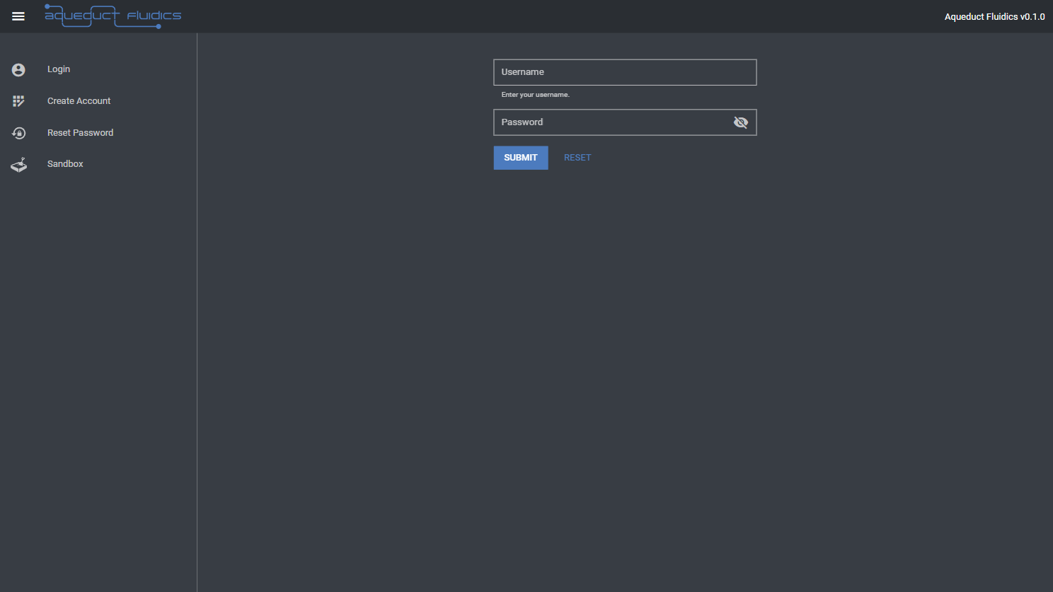
Login
The Login page in the Aqueduct dashboard allows you to securely access your account and manage your Aqueduct system.
Logging into the Dashboard
-
Open a web browser on your computer.
-
In the address bar, enter the URL for the Aqueduct Dashboard. The default URL is
http://127.0.0.1:5000, assuming you are running Aqueduct on the local machine. If you have customized the server settings, please use the appropriate IP address and port number. -
Press Enter or Return to load the Aqueduct Dashboard login page.
-
On the login page, you will see a login form.
-
Enter the following credentials to log in:
- Username: admin
- Password: password
-
After entering the credentials, click the
Submitbutton. -
If the provided credentials are correct, you will be logged into the Aqueduct Dashboard and redirected to the main dashboard interface.
-
You can now explore the various features and functionality offered by the Aqueduct Dashboard, such as managing recipes, monitoring devices, and accessing logs.
-
To log out of the Aqueduct Dashboard, look for the
Logoutbutton located at the bottom of the left side menu.
Please note that it is highly recommended that you change the default password for the admin user after the initial login. See the User Settings page for instructions on how to change your password.
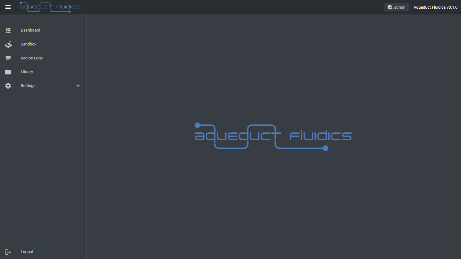
Dashboard Overview
The Dashboard page allows you to access user and public setups and recipes. The page is organized into two tabs: Setups and Recipes. Each tab displays a table with the following columns:
- Model Name: The name of the setup or recipe.
- Description: Brief description or details of the setup or recipe.
- Created On: The date and time when the setup or recipe was created.
- Actions: Provides options to activate the model in simulation or lab mode, edit the model, or delete the model.
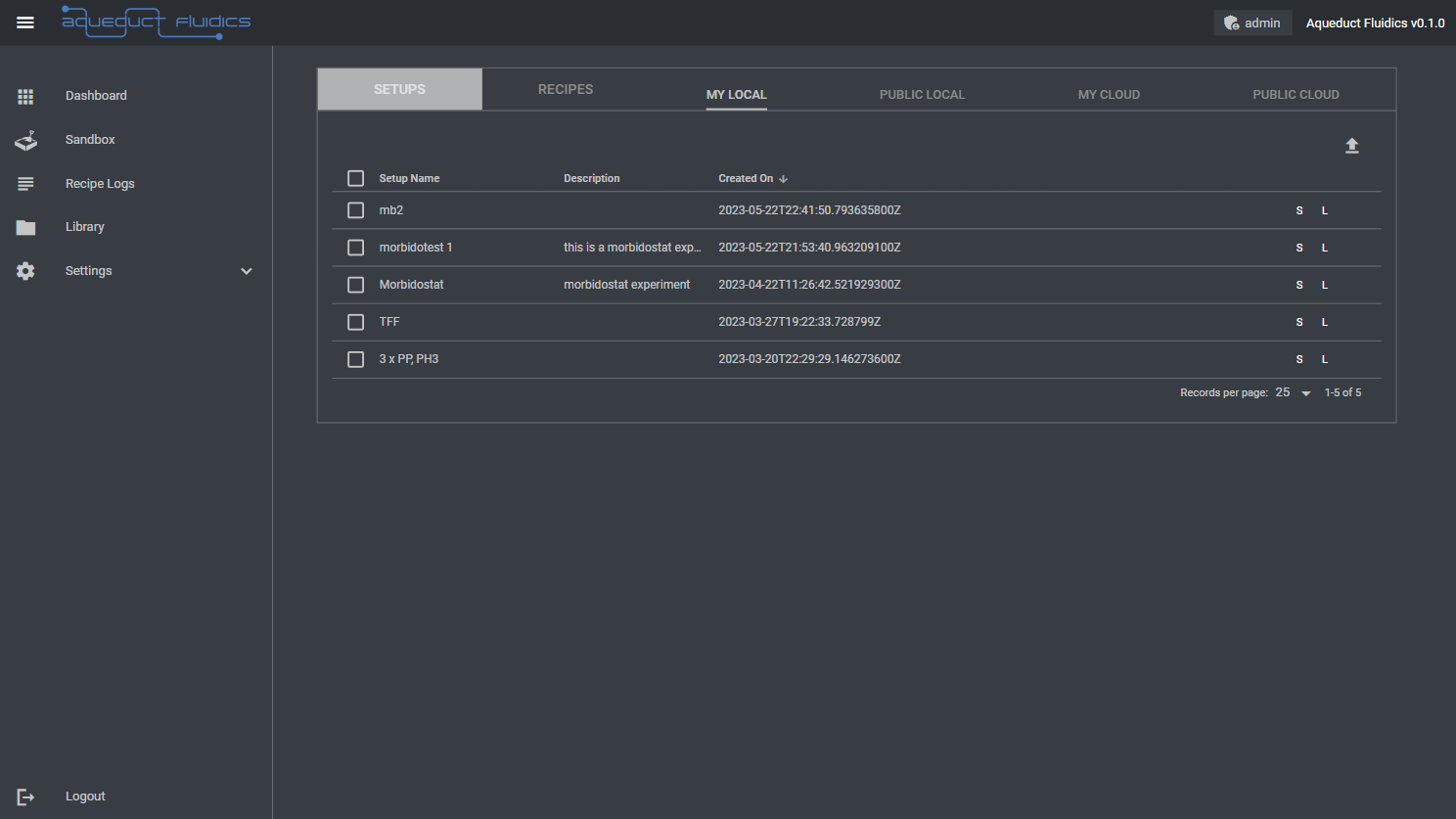
Setups or Recipes Tabs
The Setups or Recipes tab displays a table of models available in your Aqueduct application. The models are categorized into four subtabs:
- My Local: Setups or Recipes created by you.
- Public Local: Setups or Recipes shared publicly by other users.
- My Cloud: [Cloud access to setups is currently under development and not functional.]
- Public Cloud: [Cloud access to setups is currently under development and not functional.]
Accessing Models
To access setups or recipes:
-
Select the appropriate tab (Setups or Recipes) based on the model type you want to access.
-
Within the selected tab, click on the desired subtab (My Local, Public Local, My Cloud, or Public Cloud) to choose the source of the model you wish to access.
-
Locate the table row corresponding to the model you want to access.
-
Use the action buttons in the Actions column to perform specific actions on the model. These actions include activating the model in simulation or lab mode, editing the model, or deleting the model.
Please note that the availability and accessibility of models may vary based on your user permissions and the configurations set by the model authors.
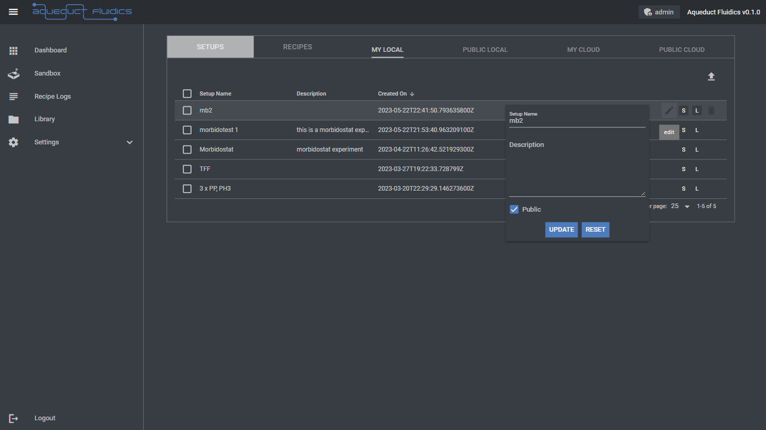
Editing Setups and Recipes
Click the pencil icon in the respective row to edit the item's details. This allows you to update the name, modify the description, or change the visibility settings of the setup or recipe.
Downloading Setups and Recipes
To download a model (setup or recipe) from the table, select the row associated with the model and click the download icon at the top right of the table. You can download a single model with the .setup or .recipe extension or multiple models archived as a .zip file. This allows you to save the model file to your local machine for further use or backup.
Uploading Setups and Recipes
To upload a model (setup or recipe) to the dashboard, click the Upload Icon button located at the top right of the table. This opens a file selection dialog where you can choose the model file (in the appropriate format) from your local machine and upload it to the dashboard. Once uploaded, the model will be available in the corresponding table. The model must have the appropriate extension (.setup or .recipe) and will be validated by the application to ensure the correct content.
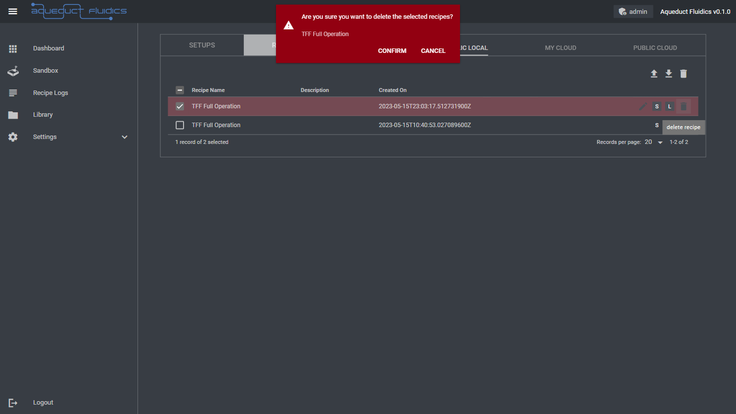
Deleting Setups and Recipes
To delete one or more models (setups or recipes) from the table, click the rows associated with the models and then click the delete icon at the top right corner of the table. You will be presented with a confirmation popup to confirm that you want to delete the selected models. This action permanently removes the models from the dashboard, so ensure that you have the necessary backups or copies if you wish to retain the models.
Sandbox Overview
The Sandbox page allows you to interact with your setup. It facilitates:
Device Interaction
- Access and control individual devices in your setup.
- Adjust settings, start or stop operations, and monitor parameters.
- Simulate device actions and observe real-time effects.
Recipe Execution
- Load and execute saved recipes.
- Observe how devices, containers, and connections interact based on defined steps.
- Test and validate recipes before real laboratory execution.
Data Monitoring
- Monitor and record data generated by devices during Sandbox interactions.
- Visualize data in real-time graphs for trend analysis and pattern identification.
- Make data-driven decisions to optimize process performance.
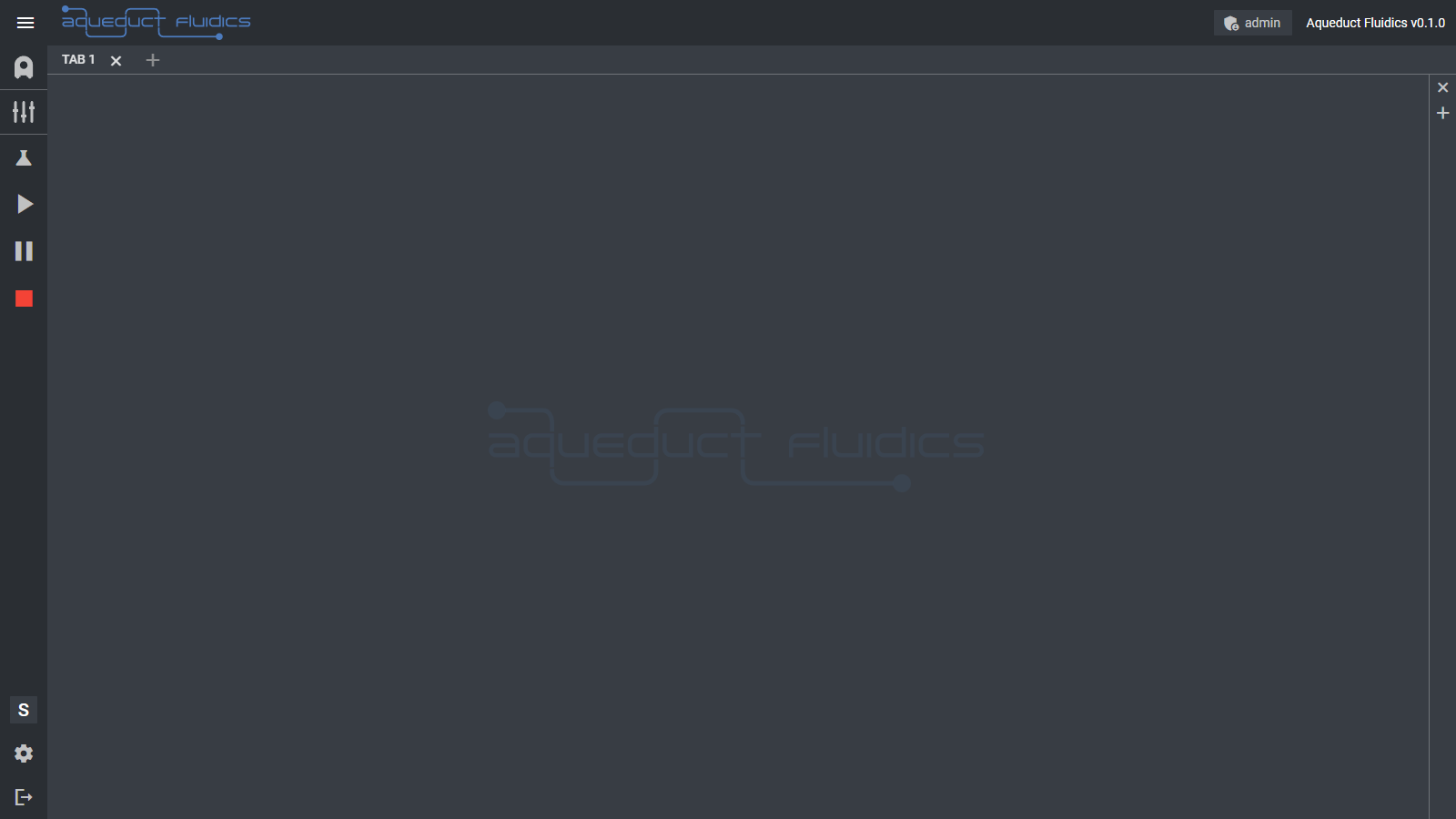
Window Arrangement and Adding a Device
We'll begin our introduction to the Sandbox by rearranging the main window workspace.
If you see a faint Aqueduct Fluidics logo on a white canvas, it means that you have an empty Tab; no Tab Containers or Widgets have been added to it yet.
Each workspace Tab can contain one or more Tab Containers. Each Tab Container can contain one or more Widgets.
Nesting Widgets in Tab Containers and Tab Containers in Tabs gives you the flexibility to organize the interface's layout to suit your application and personal preferences.
Let's add a Tab with a single, empty Tab Container to the workspace by clicking the plus icon just to the right of the left sidebar menu. Next, add a Widget to the new Tab Container by clicking the plus icon on the vertical Tab Container menu at the right of the screen. We want to add a Sandbox Widget, so click:
> Add Widget > Sandbox
The Sandbox Widget displays cartoon icons of all of the Devices, Containers, and Connections in your Setup. The icons have interactive buttons and animate to indicate activity.
Now we're ready to add a Device to our Setup, which is currently empty.
Before continuing, make sure that you're in Simulation Mode by verifying that the Mode Indicator badge on the lower left sidebar menu displays an S. If you see an L, you're in Lab Mode. Switch to Sim Mode by clicking the Settings Button (gear icon) below the badge and selecting:
> Mode > Sim
To add a Device, expand the Setup menu by clicking the Setup Menu Toggle (pump icon) on the left sidebar menu. Click the plus icon to the right of the Devices expansion menu to reveal the Device Library, which is organized by device function. Select:
> Pumps > Peristaltic Pump (PP)
to add a PP Device. A new PP Icon will appear in the Sandbox Widget and a new peristaltic_pump_000001 entry will appear in the Devices expansion menu. By default, each Simulated device is assigned the name:
[TYPE]_[NUMBER]
when it's added to the Setup, so our first peristaltic_pump type Device gets the name peristaltic_pump_000001.
We'll see how to change the name later.
You can also add a Device from the context (right click) menu in the Sandbox Widget. Right click in the widget, and then select:
Add Component > Device > Pumps > Peristaltic
to add a second peristaltic pump. We don't actually want this pump, so you can go ahead and delete it by right clicking on the icon and selecting:
Delete Device
Ok, we have a pump. Now let's see how to interact with it...
Device Control
Let's see how to control the peristaltic pump device that we've just added to our Setup.
Reveal the controls for the peristaltic pump device by clicking:
Devices > peristaltic_pump_000001 > Controls
from the Setup Menu on the left sidebar menu. You'll see some control buttons
(reverse, pause, stop, and forward), readouts for the pump's speed in mL/min and a
counter for the volume of liquid displaced, mL pumped.
Below a horizontal line are inputs for parameters that control the pump's operation. There are inputs
for a rate value, a dropdown to select the rate units, a toggle to select whether to
run the pump continuously or for a finite volume, and an input to enter an optional
finite value and finite units if finite mode is selected. For instance, if you wish to run the
pump for a defined number of milliliters or number of seconds, you would use finite mode.
Enter 10 in the field for mL/min and click the right (forward) arrow to start the pump.
The pump is now operating continuously in the clockwise direction at 10 mL/min. You should
see the mL pumped display counter increase with time as the pump displaces more (simulated)
liquid.
When you're ready to stop the pump, press the stop button. You should see the rollers on the
icon stop rotating and the mL/min display in the control window reset to 0 mL/min.
Next, click the left (reverse) arrow to start the pump in the opposite direction. Again, the
mL pumped display counter increases with time as the pump continues to run.
You probably noticed that there are also buttons above the peristaltic pump Icon in the Sandbox Widget. If they're not visible, toggle control visibility by opening the Sandbox context menu (right click) and select:
Display > Controls > Show
These buttons function in the same way as the buttons in the Control Panel and will use the
same parameters that are entered in the Panel. Let's use these buttons to run the pump for
1 milliliter in the forward direction at 10 mL/min. Toggle the vertical mode selector to finite, enter
10 in the units entry and make sure that mL is selected in the dropdown.
Now, press the forward button above the peristaltic pump icon in the Sandbox Widget.
Again, the pump will start running, but you'll notice that once the mL pumped display
reaches 1 milliliter, the pump will stop.
Summary: Device Interactions in the Aqueduct User Interface
The Aqueduct User Interface provides a consistent and intuitive approach to interact with devices. Whether you are controlling a peristaltic pump, a temperature controller, or any other device, the following key points summarize the device interactions in the Aqueduct User Interface:
-
Accessing Device Controls: Navigate to the Devices section in the Setup Menu on the left sidebar. Expand the device of interest to reveal the sub-menu, and click on Controls to access the specific controls and parameters for that device.
-
Inputting Device Parameters: Adjust the device's parameters using the provided controls, buttons, and input fields. Common parameters include rate values, unit selections, mode toggles (continuous or finite), and optional finite values and units.
-
Multiple Nodes per Device: In some cases, a device may have multiple nodes associated with it, such as multiple channels in a peristaltic pump. A master node controls the operation of all associated nodes. Starting or stopping the master node synchronizes the actions across all nodes within the device.
-
Sandbox Icon Buttons and Parameters: The Sandbox Widget allows direct device control. Right-click on the Sandbox Widget to access the context menu and select Display > Controls > Show to reveal the buttons associated with each device icon. These buttons function the same way as the controls in the Setup Menu and utilize the parameters entered in the Controls section.
When you're finished running the simulated pump actions, move on to the the next step, where we'll add some Containers and Connections to help us visualize and document the Setup.
Add Containers and Make Connections
So now we have a pump that we can run clockwise or counterclockwise for an indefinite (continuous) or finite duration. Next, let's add some Containers - simulated vessels - to serve as a source and sink for the pump to transfer liquid from/to.
Why add Containers? You certainly don't need to, and you can script Recipes with only Devices, but Containers (and Connections, which are coming next) can be a helpful visualization tool for recreating a Setup in the lab and for intuiting your Setup in the Sandbox.
Adding a Container follows the same steps as adding a Device. Expand the Setup menu by clicking the Setup Menu Toggle (pump icon) on the left sidebar menu. Click the plus icon to the right of the Containers expansion menu to reveal the Container Library. Select:
> Containers > Bottles > 100 mL Bottle
to add a new 100 mL bottle to the setup. A new Bottle Icon will appear in the Sandbox Widget and a new 100 mL bottle entry will appear in the Containers expansion menu. By default, each container is assigned its type (100 mL bottle, in this case) as its name when it's added to the Setup.
Just like Devices, you can also add a Container from the context (right click) menu in the Sandbox Widget. Right click in the widget, and then select:
Add Component > Container > Bottles > 100 mL bottle
Add two 100 mL bottles using whichever method you prefer. Drag them into a reasonable position below the peristaltic pump Device by clicking the wall of the icon and dragging.
Now, let's make Connections - our digital representation of tubing - between the new bottles and our pump. Connections are added by clicking on Ports, which appear as gray circles. Ports represent a physical tubing connection mechanism, like a port, a barbed fitting, or any other mechanism that joins a length of tubing to a Device or Container.
After each Port click, you'll see a blue notification confirming the Device or Container name and port number that you've selected and confirmation that the new connection has been added. A new connection key entry will appear in the Connections expansion menu, which should read something like U:000. *U indicates that the connection was made by the user (it does not belong to a Device or Container), and the digits 000 are the connection's index.
Unlike Devices and Containers, Connections cannot be renamed.
All right, we have a basic Setup: a pump (peristaltic pump Device), two bottles, and two connections linking the pump and containers. Let's proceed to see how to save this Setup on the Hub, clear the Setup, and then reload our Setup to script a Recipe.
Saving, Clearing, and Reloading
At this point, we've added the Devices and Containers that we need for our demo, arranged them on the Sandbox Widget, and added two Connections. We want to save this configuration as a Setup so we can reuse it later without having to rebuild it.
Before we do that, let's rename our PP Device to something other than the default name peristaltic_pump_000001. Understanding how Device names impact their accessibility in Recipes is important, and we'll address that when we script our Recipe. For now, pick any name you like, then right click on the device menu label to reveal a context menu:
Config > Base
and enter the name.
Once a change has been made, click update all to save your changes.
Now we're ready to save our Setup. The Save Setup menu is accessible from both the Sandbox Widget menu (the ellipsis icon at the top left of the widget) and the context (right click) menu. Use whichever method you wish, then select:
> Save Setup
A form with entries for a Setup Name and Description and a toggle for Public will appear.
The Setup Name is the name that will appear in your list of saved Setups, the Description is an
entry for adding more detail about the Setup, and the Public toggle controls whether the Setup will
be visible to other Users. (This does not mean that it's available via the internet but
only that it's available locally.)
After we click Save, we receive a notification indicating that we've successfully saved our new first setup.
Now, let's see how we can reload the Setup. First, we'll clear the Setup - all of our Devices, Containers, and Connections - by using the Sandbox Widget menu or the context menu to select:
> Clear Setup > Confirm
from the Sandbox Widget menu. Our icons will disappear from the Sandbox and the names of our Devices and Containers will be removed from the Setup expansion menus.
When we're ready to use this Setup again, we can reload it to our saved state by using the Sandbox menu to select:
> Load Setup > My Local > test setup > S
Because we own this Setup (we created it), it's displayed in the My Local submenu. We select the S to activate the Setup in Sim Mode. Clicking the S starts the activation procedure and a blue notification appears at the top of the screen with status updates. Upon completion, you should see a success message in the notification and your icons will reappear in the Sandbox.
So, we've successfully saved, cleared, and reloaded our first Setup. Now let's move beyond manual control and write a Recipe script to control the pump automatically.
Recipe Creation
Aqueduct Recipes are written in Python (3.7+). Python's powerful standard library gives you great flexibility in implementing your Recipe's logic and data management, but you must have some familiarity with Python to begin scripting.
There are many excellent introductions and tutorials for Python available, including:
so we won't attempt to provide a full introduction here. Instead, we'll focus on Python in the context of the Aqueduct environment.
Limitations
When using the Aqueduct environment, you have the flexibility to run the Python recipe process on the same host as the core application or on another computer. The communication between the Python process and the Aqueduct application is established through a TCP socket interface.
The Aqueduct library registers the Python process with the Aqueduct application. This registration allows the Aqueduct user interface (UI) to interact with the Python process. The UI can pause and resume the process, as well as send updates of device data to the Python process.
This capability enables seamless integration between the Aqueduct UI and the Python process, allowing for real-time control, monitoring, and data exchange. Whether running the Python process on the same host or a different computer, the Aqueduct environment ensures synchronized communication and efficient coordination between the application and the Python code.
Please note that when running the Python process on a separate computer, appropriate network configuration and access permissions are required to establish the TCP socket connection between the host and the Aqueduct application.
Adding the Recipe Editor and Terminal Widgets
Ok, with those caveats out of the way, let's start writing a Recipe for our Setup. First, let's add the Recipe Editor Widget to our window.
Again, click the plus icon on the vertical Container menu at the right of the screen. This time select:
> Add Widget > Recipe > Editor
You'll see a new Widget appear to the right of the Sandbox Widget. The Editor Widget lets you enter Python code directly in the interface.
While we're rearranging, let's add another Widget - the Output Widget - to our layout. The
Recipe Output widget will output any print statements that you execute during your Recipe. Instead of
being directed to your local interpreter's standard output, the print output is pushed to the
Terminal Widget in the interface. Select:
> Add Widget > Recipe > Output
To keep things neat, let's add another Tab Container to our layout to house the Editor and Terminal. Click the plus icon on the vertical Container menu and select:
> Add Container After
Then, drag the Editor and Terminal Widgets to the new Container by selecting their menu bars and dragging them to the new Tab Container. You can change the layout of a Tab's Containers by selecting the gear icon on the left sidebar menu, then clicking:
> Layout > Columns
This will change the arrangement of the Tab so that the Containers are oriented as vertical columns. In this case, we have two Tab Containers, one housing the Sandbox Widget and one housing the Editor and Terminal Widgets.
You can also change the Layout of a Container by selecting the plus menu, then selecting:
> Row Layout
This will arrange the Widgets within the container as rows spanning the entire width.
Now let's move on to see how we can write code that will control the pump's operation and execute our recipe...
Use the API
To interact with and control Devices in an Aqueduct Recipe, you'll make use of the
aqueduct-py API. The API is a collection of Python Classes and Methods that
you can leverage to control Recipe execution, generate User Inputs and Prompts,
visualize data, and control Devices.
Each Device type has an associated Python class with the same name. So, our
peristaltic pump device will use the PeristalticPump class in the Aqueduct API. You
can see the source code for the different device types in the aqueduct-py repository here devices and the PeristalticPump specifically here: peristaltic.py.
Registering a Python Process and Loading Devices
To interact with the Aqueduct system and control the devices in your Setup, you need to register your Python process with the Aqueduct application. This registration is done using the following lines of code:
from aqueduct.core.aq import Aqueduct
from aqueduct.core.aq import InitParams

# parse initialization parameters and create Aqueduct instance
params = InitParams.parse()
aq = Aqueduct(params.user_id, params.ip_address, params.port)

aq.initialize(params.init)
After registering your recipe, you can access the devices in your Setup by their names. For example, to retrieve the peristaltic pump named peristaltic_pump_000001, use the following code:
from aqueduct.devices.pump import PeristalticPump
pump: PeristalticPump = aq.devices.get("peristaltic_pump_000001")
print(pump)
Copy the text into the editor. Now, let's queue our Recipe by using the Editor Widget menu (the ellipsis) to select:
> Queue Recipe
You'll receive a notification saying that the Recipe was successfully queued and the Recipe Status Indicator will display a blue Q. Click the Start/Resume Recipe Button on the left sidebar menu to start the Recipe.
The output in the Recipe Output Widget reads:
<aqueduct.devices.pump.peristaltic.PeristalticPump object at 0xb4b0fb90>
The printable representation shows that we have a aqueduct.devices.pump.peristaltic.PeristalticPump object at some location
in memory 0xb4b0fb90.
You've run your first recipe! After the recipe is complete, the Recipe Status Indicator displays a blue C indicating that it's complete. This recipe didn't do anything useful, but these are the basics of scripting in the Aqueduct environment.
- Enter your Recipe Script in the Editor Widget
- Queue your Recipe
- Press the Start/Resume Recipe Button to begin execution
Creating and Sending Device Commands
Now let's write a recipe that:
- starts the pump at 2 mL/min
- changes its speed in a loop up to 50 rpm by an increment of 0.1 mL/min
- then decrements its speed to 0.1 mL/min
- and then stops the pump
Let's use our previous snippet as a starting point:
from aqueduct.core.aq import Aqueduct
from aqueduct.core.aq import InitParams
from aqueduct.devices.pump import PeristalticPump

# parse initialization parameters and create Aqueduct instance
params = InitParams.parse()
aq = Aqueduct(params.user_id, params.ip_address, params.port)

# initialize the devices and set a command delay
aq.initialize(params.init)
aq.set_command_delay(0.05)

# get the peristaltic pump device and create a command object
pump: PeristalticPump = aq.devices.get("peristaltic_pump_000001")

# todo - start pump

# set the maximum speed and speed increment for the pump
MAX_SPEED: float = 50
INCREMENT: float = 0.1

# calculate the number of steps based on the maximum speed and increment
STEPS = int(MAX_SPEED / INCREMENT)

# loop through the speed increment steps
for i in range(0, STEPS):
    # todo
    _ = i

# loop through the speed decrement steps
for i in range(STEPS, 0, -1):
    # todo
    _ = i

# todo - stop pump
The first action we need to implement in the script is starting the pump.
To control a device in the Aqueduct system, you can create commands that specify the desired settings and actions for the device.
First, create an empty list to store the commands for the pump:
commands = pump.make_commands()
Next, create a specific command to start the pump. In this example, we want the pump to run continuously at a rate of 2 mL/min in the clockwise direction. The make_start_command() method is used to create the command with the desired settings:
command = pump.make_start_command(
    mode=pump.MODE.Continuous,
    rate_units=pump.RATE_UNITS.MlMin,
    rate_value=2,
    direction=pump.STATUS.Clockwise,
)
Once the command is created, you can set it for the pump. Since there may be multiple nodes or channels in a pump, you need to specify the index of the node for which you want to set the command. In this case, we are using the first (and only) node, which has an index of 0:
pump.set_command(commands, 0, command)
Finally, send the start command to the Aqueduct system to initiate the pump operation:
pump.start(commands)
These steps allow you to create and set commands for controlling devices in the Aqueduct system. By specifying the desired settings and actions in the commands, you can effectively operate and control the devices according to your requirements.
from aqueduct.core.aq import Aqueduct
from aqueduct.core.aq import InitParams
from aqueduct.devices.pump import PeristalticPump

# parse initialization parameters and create Aqueduct instance
params = InitParams.parse()
aq = Aqueduct(params.user_id, params.ip_address, params.port)

# initialize the devices and set a command delay
aq.initialize(params.init)
aq.set_command_delay(0.05)

# get the peristaltic pump device and create a command object
pump: PeristalticPump = aq.devices.get("peristaltic_pump_000001")

# make an empty commands list
commands = pump.make_commands()

command = pump.make_start_command(
    mode=pump.MODE.Continuous,
    rate_units=pump.RATE_UNITS.MlMin,
    rate_value=2,
    direction=pump.STATUS.Clockwise,
)

# set the command for the first (and only) node of the pump
pump.set_command(commands, 0, command)

# now send the start command
pump.start(commands)

# set the maximum speed and speed increment for the pump
MAX_SPEED: float = 50
INCREMENT: float = 0.1

# calculate the number of steps based on the maximum speed and increment
STEPS = int(MAX_SPEED / INCREMENT)

# loop through the speed increment steps
for i in range(0, STEPS):
    # todo
    _ = i

# loop through the speed decrement steps
for i in range(STEPS, 0, -1):
    # todo
    _ = i

# todo - stop pump
At this point, let's queue up our edited script and run it:
The pump starts and our recipe completes, as shown by the Recipe Status Indicator displaying a blue C.
Now we're ready to add logic to ramp up and
then ramp down the pump's speed. We'll use two for loops - one loop to count up in
a configurable increment to our target top speed (50 mL/min), and one loop to decrement
from our top speed to our ending speed (2 mL/min).
To avoid duplicating parameters,
we'll create the variables MAX_SPEED, INCREMENT, and STEPS
to define these values in a single place in the code. Additionally, we'll add a
print statement in each loop to confirm that we're hitting our targets, as the pump display
may not update quickly enough to give us feedback.
commands = pump.make_commands()

command = pump.make_start_command(
    mode=pump.MODE.Continuous,
    rate_units=pump.RATE_UNITS.MlMin,
    rate_value=2,
    direction=pump.STATUS.Clockwise,
)

# set the command for the first (and only) node of the pump
pump.set_command(commands, 0, command)

# now send the start command
pump.start(commands)

# set the maximum speed and speed increment for the pump
MAX_SPEED: float = 50
INCREMENT: float = 0.1

# calculate the number of steps based on the maximum speed and increment
STEPS = int(MAX_SPEED / INCREMENT)

# ramp up the speed to `top_speed_rpm`
for i in range(0, STEPS):
    commands = pump.make_commands()

    # create a command to change the pump speed
    c = pump.make_change_speed_command(
        rate_value=i * INCREMENT, rate_units=pump.RATE_UNITS.MlMin
    )

    pump.set_command(commands, 0, c)

    pump.change_speed(commands)

    print(f"Ramping up to: {i * INCREMENT} mL/min")

# ramp down the speed to `2 mL/min`
for i in range(STEPS, 0, -1):
    commands = pump.make_commands()

    # create a command to change the pump speed
    c = pump.make_change_speed_command(
        rate_value=i * INCREMENT, rate_units=pump.RATE_UNITS.MlMin
    )

    pump.set_command(commands, 0, c)

    pump.change_speed(commands)

    print(f"Ramping down to: {i * INCREMENT} mL/min")

# todo
Our recipe logic is almost there; we just need to stop the pump after the ramp down to 2 mL/min has
completed. Let's modify the script to call the PeristalticPump class's stop method
at the end of the script:
from aqueduct.core.aq import Aqueduct
from aqueduct.core.aq import InitParams
from aqueduct.devices.pump import PeristalticPump

# parse initialization parameters and create Aqueduct instance
params = InitParams.parse()
aq = Aqueduct(params.user_id, params.ip_address, params.port)

# initialize the devices and set a command delay
aq.initialize(params.init)
aq.set_command_delay(0.05)

# get the peristaltic pump device and create a command object
pump: PeristalticPump = aq.devices.get("peristaltic_pump_000001")

commands = pump.make_commands()

command = pump.make_start_command(
    mode=pump.MODE.Continuous,
    rate_units=pump.RATE_UNITS.MlMin,
    rate_value=2,
    direction=pump.STATUS.Clockwise,
)

# set the command for the first (and only) node of the pump
pump.set_command(commands, 0, command)

# now send the start command
pump.start(commands)

# set the maximum speed and speed increment for the pump
MAX_SPEED: float = 50
INCREMENT: float = 0.1

# calculate the number of steps based on the maximum speed and increment
STEPS = int(MAX_SPEED / INCREMENT)

# ramp up the speed to `top_speed_rpm`
for i in range(0, STEPS):
    commands = pump.make_commands()

    # create a command to change the pump speed
    c = pump.make_change_speed_command(
        rate_value=i * INCREMENT, rate_units=pump.RATE_UNITS.MlMin
    )

    pump.set_command(commands, 0, c)

    pump.change_speed(commands)

    print(f"Ramping up to: {i * INCREMENT} mL/min")

# ramp down the speed to `2 mL/min`
for i in range(STEPS, 0, -1):
    commands = pump.make_commands()

    # create a command to change the pump speed
    c = pump.make_change_speed_command(
        rate_value=i * INCREMENT, rate_units=pump.RATE_UNITS.MlMin
    )

    pump.set_command(commands, 0, c)

    pump.change_speed(commands)

    print(f"Ramping down to: {i * INCREMENT} mL/min")

pump.stop() ## <---------- stop
print("Complete!")
Queue and rerun: (Rearrange your window if needed to make the Terminal output visible.)
Very nice. We've successfully implemented the steps we outlined earlier. Let's move on to see how to interact with an active Recipe.
Pause and E-Stop
Most of your Recipes won't be as short or simple as our ramp up and ramp down demo. They may run for extended periods of time and you may find that you need to pause and resume your recipe prior to completion.
While a Recipe is active - Running, Paused, or E-Stopped - you can use the Recipe Control Buttons on the left sidebar menu to control the Recipe's state.
Let's see an example of interacting with a Recipe by writing a quick
script for a Recipe that will never complete on its own. Let wrap the loop logic in our previous
recipe in a while True: ... loop that will never return - it will
run in a loop forever and change the pump's speed from 0 mL/min to 50 mL/min in
each loop iteration.
from aqueduct.core.aq import Aqueduct
from aqueduct.core.aq import InitParams
from aqueduct.devices.pump import PeristalticPump

# parse initialization parameters and create Aqueduct instance
params = InitParams.parse()
aq = Aqueduct(params.user_id, params.ip_address, params.port)

# initialize the devices and set a command delay
aq.initialize(params.init)
aq.set_command_delay(0.05)

# get the peristaltic pump device and create a command object
pump: PeristalticPump = aq.devices.get("peristaltic_pump_000001")

commands = pump.make_commands()

command = pump.make_start_command(
    mode=pump.MODE.Continuous,
    rate_units=pump.RATE_UNITS.MlMin,
    rate_value=2,
    direction=pump.STATUS.Clockwise,
)

# set the command for the first (and only) node of the pump
pump.set_command(commands, 0, command)

# now send the start command
pump.start(commands)

# set the maximum speed and speed increment for the pump
MAX_SPEED: float = 50
INCREMENT: float = 1

# calculate the number of steps based on the maximum speed and increment
STEPS = int(MAX_SPEED / INCREMENT)

while True:  ## <---------- infinite loop
    # ramp up the speed to `top_speed_rpm`
    for i in range(0, STEPS):
        commands = pump.make_commands()

        # create a command to change the pump speed
        c = pump.make_change_speed_command(
            rate_value=i * INCREMENT, rate_units=pump.RATE_UNITS.MlMin
        )

        pump.set_command(commands, 0, c)

        pump.change_speed(commands)

        print(f"Ramping up to: {i * INCREMENT} mL/min")

    # ramp down the speed to `2 mL/min`
    for i in range(STEPS, 0, -1):
        commands = pump.make_commands()

        # create a command to change the pump speed
        c = pump.make_change_speed_command(
            rate_value=i * INCREMENT, rate_units=pump.RATE_UNITS.MlMin
        )

        pump.set_command(commands, 0, c)

        pump.change_speed(commands)

        print(f"Ramping down to: {i * INCREMENT} mL/min")

pump.stop()
print("Complete!")
Copy and paste the above code into the Editor Widget, queue the Recipe, and begin execution. You'll see the pump cycling between 0 and 50 mL/min.
Pausing a Recipe
We can Pause execution of our Recipe by pressing the Pause Recipe Button on the left sidebar menu:
| Pause Recipe Button |

|
The Paused state indicates that your Recipe's Python process is active but has been temporarily paused to prevent further execution. The Recipe Status Indicator will display a yellow P badge:
| Paused Recipe Status Indicator |

|
The Recipe transitions into the Paused state without any further input needed from the user and no Device actions are executed when a Recipe is paused.
Devices are left in the same state as they were in before the Pause Recipe Button was pressed. Notice that peristaltic_pump_000001 continued to operate at 12.5 mL/min.
To resume the Recipe, simply click the Start/Resume Recipe Button:
| Start/Resume Recipe Button |

|
The Recipe will pick back up where it left off and peristaltic_pump_000001 will continue to cycle between 0 and 50 mL/min.
Emergency Stopping a Recipe
We can also issue an E-Stop command to our Recipe by pressing the E-Stop Recipe Button on the left sidebar menu:
| E-Stop Recipe Button |

|
Just like Pausing your Recipe, E-Stopping pauses execution of your Recipe's Python process to prevent further execution.
However, an E-Stop command also issues stop commands to all Devices that are considered active when the E-Stop button is pressed. Active devices, such as operating pumps or robotic arms, are issued commands to stop any motion. Passive devices, such as balances, pH probes, or other sensors that simply transmit data and do not move, are left unaffected.
The Recipe Status Indicator will display a yellow ES badge:
| E-Stopped Recipe Status Indicator |

|
Notice that peristaltic_pump_000001 stopped operating when we pressed the E-Stop Recipe Button.
To resume the Recipe, click the Start/Resume Recipe Button. Because the Recipe is re-entering the Running state from the E-Stopped state, we will be asked to select which Devices are to resume operation before the Python process is restarted.
The Resume Recipe dialog displays a table with one or more rows for each Device. Each row specifies the action(s) that will be taken by default for that Device when the Recipe resumes, restoring the Device to the state it was in when the E-Stop button was pressed.
To ignore the default action, deselect the checkbox in the Resume? column.
Interacting with Devices while a Recipe is Paused or E-Stopped
All manual Device commands are accessible while a Recipe is Paused or E-Stopped.
You are free to use the controls from the Setup Menu on the left sidebar menu that we discussed in the Device Control section to manually control Devices as needed.
The following clip illustrates this functionality by:
- Pausing our infinite Recipe using the Pause Recipe Button
- Manually stopping peristaltic_pump_000001 using the Sandbox Widget stop button
- Running peristaltic_pump_000001 in
continuousmode at10 mL/minin theclockwisedirection using the controls parameter inputs - Resuming the infinite Recipe using the Start/Resume Recipe Button
Wrapping Up
In summary, the basics of interacting with an active recipe are:
- Pausing a Recipe temporarily stops execution of the Recipe's Python process without affecting the state of any Devices
- E-Stopping a Recipe temporarily stops execution of the Recipe's Python process AND stops any active Devices
- All manual Device commands - the buttons accessible on the left sidebar menu and the buttons associated with a Device in the Sandbox Widget - remain accessible when a Recipe is Paused or E-Stopped
Now, let's continue to build on our infinite while loop script...
Data Visualization and Recording
Often, you'll want access to historical data generated by Devices in addition to seeing data about their current states. Most Devices in the Aqueduct Library have the ability to record their state at each update interval. These recorded timeseries can be visualized in the user interface with a Chart Widget.
Let's add a new Tab and Tab Container to our window and then add a Chart Widget:
A Chart Widget allows you to view Recordable timeseries for both Device and User data. We'll see how to create a User Recordable later, but for now let's add a Device Recordable to the Chart by selecting:
> Series > Devices > peristaltic_pump_000001 > pump 0 disp. (mL)
Use the controls section in the left menu to start peristaltic_pump_000001 in the clockwise direction at 10 mL/min. Make sure that the checkbox in the record toggle is selected and then press the start button on the control panel:
As the pump starts operating, you'll see a line appear on the chart that increases with time. We're plotting the milliliters displaced by the pump.
Enter a larger rate value (20 mL/min, for instance) in the controls panel and
press the start button again. The milliliters displaced value will reset to 0 and then start
increasing at a higher rate.
You can add multiple Chart Widgets to your window layout. Add a second Chart Widget to the Tab Container and then add the pump 0 rate (mL/min) timeseries.
Let's revisit our infinite loop recipe from the last step and modify it to
record the changes in the pump's rate. The only change that we need to make is
the addition of setting the record argument to True in the pump's start method:
pump.start(commands, record = True)
You'll see a record argument in many Device methods throughout the
Aqueduct API. The functionality of this argument is the same:
setting record to True will instruct the platform to record
the device's state in a timeseries and make it accessible in Chart Widgets.
Make the above change to your code in the Editor Widget, queue the Recipe, and begin execution. Now, in addition to seeing the pump cycling between 0 and 50 mL/min, you'll see a sawtooth-like timeseries of the pump's rpm as our Recipe continuously changes its speed.
You can create your own timeseries
using the Aqueduct API's Recordable class. For instance, you may wish to calculate a
derived value using device data as an input.
Let's make a Recordable to display the total volume displaced by the pump during our Recipe. Go
back to the PeristalticPump class in the Aqueduct API (peristaltic.py) and take a look at the get_ml_done method:
aqueduct/devices/pump/peristaltic.py
class PeristalticPump(devices.base.obj.Device):

    # snip

    def get_ml_done(self) -> Tuple[float]:
        """
        Get the volume dispensed by the peristaltic pump in milliliters.

        :return: Volume dispensed in milliliters.
        :rtype: tuple
        """
        return self.extract_live_as_tuple(PeristalticPumpLiveKeys.ml_done.value)

    ## snip
We can use the pump's get_ml_done method to calculate volume displaced in milliliters.
The other tool we'll need to implement our volume counter is the Recordable API, which is found here (Recordable) and here (Aqueduct recordable method):
The API methods are reproduced below for easier reference:
aqueduct/core/aq.py
class Aqueduct(object):

  # snip

  def recordable(
        self,
        name: str,
        value: typing.Union[float, int, bool, str, datetime.datetime, list],
        dtype: str = None,
    ) -> Recordable:
        """
        Creates a new Recordable object and registers it with Aqueduct.

        :param name: The name of the Recordable.
        :type name: str
        :param value: The initial value of the Recordable.
        :type value: Union[float, int, bool, str, datetime.datetime, list]
        :param dtype: The data type of the Recordable value, defaults to None.
        :type dtype: str, optional
        :return: The newly created Recordable object.
        :rtype: Recordable
        """
        recordable = Recordable(name, value, dtype)
        self.register_recordable(recordable)
        self.update_recordable(recordable)
        return recordable

  # snip
aqueduct/core/recordable.py
class Recordable:
    """
    The `Recordable` class allows you to log timestamped data.

    :param name: Name of the recordable, will be displayed on the UI, should be unique
    :type name: str, required
    :param value: Initial value to be assigned to the recordable on creation
    :type value: float, int, bool, str, datetime.datetime, list, required
    :param dtype: Specify the type of value, used to ensure that users cannot
        enter an invalid value
    :type dtype: {'int', 'float', 'bool', 'list', 'datetime', 'str'}, optional
    """

    name: str = None
    value: Union[float, int, bool, str, datetime.datetime, list] = None
    dtype: str = None
    timestamp = None

    _aq: "Aqueduct" = None

    def __init__(
        self,
        name: str,
        value: Union[float, int, bool, str, datetime.datetime, list],
        dtype: str = None,
    ):
        """
        Constructor method.

        :param name: name of the Recordable, will be displayed on the UI, should be unique
        :type name: str, required
        :param value: value to be assigned to the Recordable on creation
        :type value: float, int, bool, str, datetime.datetime, list, required
        :param dtype: specify the type of value, used to ensure that users cannot enter an invalid value
        :type dtype: {'int', 'float', 'bool', 'list', 'datetime', 'str'}, optional
        """
        if dtype is None:
            try:
                dtype = type(value).__name__
                if dtype not in ALLOWED_DTYPES:
                    raise ValueError(
                        "Object of type {} is not allowed as a Recordable".format(
                            {dtype}
                        )
                    )
            except Exception:
                raise ValueError("Invalid Aqueduct Recordable")

        self.name = name
        self.value = value
        self.dtype = dtype

    # not all methods present

    def assign(self, aqueduct: "Aqueduct"):
        """
        Assigns the Recordable to an `Aqueduct` instance.

        :param aqueduct: The `Aqueduct` instance to assign the Recordable to.
        :type aqueduct: Aqueduct, required
        """
        self._aq = aqueduct

    def update(self, value):
        """
        Updates the value of the Recordable.

        :param value: The new value for the Recordable.
        :type value: Union[float, int, bool, str, datetime.datetime, list], required
        """
        self.value = value
        self._aq.update_recordable(self)

    def clear(self):
        """
        Clears the value of the Recordable.
        """
        self._aq.clear_recordable(self)
So, our strategy will be to create a Recordable instance using the aqueduct object's
recordable method, assign it a name of our choosing, and then update it as needed with the
value returned from the pump's ml_pumped method.
Let's modify our code to create the Recordable before the entry to our infinite loop and
update the value at the end of each loop iteration:
from aqueduct.core.aq import Aqueduct
from aqueduct.core.aq import InitParams
from aqueduct.devices.pump import PeristalticPump

# parse initialization parameters and create Aqueduct instance
params = InitParams.parse()
aq = Aqueduct(params.user_id, params.ip_address, params.port)

# initialize the devices and set a command delay
aq.initialize(params.init)
aq.set_command_delay(0.05)

# get the peristaltic pump device and create a command object
pump: PeristalticPump = aq.devices.get("peristaltic_pump_000001")

volume_pumped = aq.recordable(        ## <--- added recordable creation
  name="ml_pumped",                   ## <--- name will be displayed on chart Widget
  dtype=float.__name__,               ## <--- define the data type
  value=0.,                           ## <--- set the initial value
)

commands = pump.make_commands()

command = pump.make_start_command(
    mode=pump.MODE.Continuous,
    rate_units=pump.RATE_UNITS.MlMin,
    rate_value=2,
    direction=pump.STATUS.Clockwise,
)

# set the command for the first (and only) node of the pump
pump.set_command(commands, 0, command)

# now send the start command
pump.start(commands)

# set the maximum speed and speed increment for the pump
MAX_SPEED: float = 50
INCREMENT: float = 1

# calculate the number of steps based on the maximum speed and increment
STEPS = int(MAX_SPEED / INCREMENT)

while True:
    # ramp up the speed to `top_speed_rpm`
    for i in range(0, STEPS):
        commands = pump.make_commands()

        # create a command to change the pump speed
        c = pump.make_change_speed_command(
            rate_value=i * INCREMENT, rate_units=pump.RATE_UNITS.MlMin
        )

        pump.set_command(commands, 0, c)

        pump.change_speed(commands)

        volume_pumped.update(pump.get_ml_done()[0]) ## <--- update the value

        print(f"Ramping up to: {i * INCREMENT} mL/min")

    # ramp down the speed to `2 mL/min`
    for i in range(STEPS, 0, -1):
        commands = pump.make_commands()

        # create a command to change the pump speed
        c = pump.make_change_speed_command(
            rate_value=i * INCREMENT, rate_units=pump.RATE_UNITS.MlMin
        )

        pump.set_command(commands, 0, c)

        pump.change_speed(commands)

        volume_pumped.update(pump.get_ml_done()[0]) ## <--- update the value

        print(f"Ramping down to: {i * INCREMENT} mL/min")

pump.stop()
print("Complete!")
Let's Queue and rerun the script. After starting, navigate to the tab with your
Chart Widgets and add the ml_pumped series by selecting:
> Series > User > ml_pumped
from the Chart context menu. You should see a second timeseries with a line that continues to increase as the pump traverses more revolutions.
Looks good!
This Chapter has introduced us to Recordables and recording data, which make timeseries
data available to plot in a Chart Widget. Many device API methods accept a record argument
that will instruct the application to record that device's state at each update interval. User Recordables
can be used to extend the built-in device recording parameters with derived or calculated values
that you may wish to record over time.
Now, let's move on to the next Chapter, which will introduce Setpoints and Logging.
Setpoints and Logging
Currently, our Recipe runs forever. We've wrapped our pump ramp up/ramp down
logic in an infinite while True loop. You'll likely want your Recipe to end or at
least be able to terminate it on demand! More generally, it would be nice to have a way to
adjust parameters in our Recipe logic from the user interface in real-time. To do this,
we can use the Aqueduct Setpoint API.
The Setpoint API can be found here (Setpoint)
and here (Aqueduct setpoint method):
The API methods are reproduced below for easier reference:
aqueduct/core/aq.py
class Aqueduct(object):

  # snip

  def setpoint(
        self,
        name: str,
        value: typing.Union[float, int, bool, str, datetime.datetime, list],
        dtype: str = None,
    ) -> Setpoint:
        """
        Creates a new Setpoint object.

        :param name: The name of the setpoint
        :type name: str
        :param value: The initial value of the setpoint
        :type value: typing.Union[float, int, bool, str, datetime.datetime, list]
        :param dtype: The data type of the setpoint value, defaults to None
        :type dtype: str, optional
        :return: A new Setpoint object
        :rtype: aqueduct.core.setpoint.Setpoint
        """
        s = Setpoint(name, value, dtype)
        self.register_setpoint(s)
        self.update_setpoint(s)
        return s

  # snip
aqueduct/core/setpoint.py
class Setpoint:
    """
    A class to provide simple interaction with Recipe values that
    appear as User Params on the Aqueduct Recipe Builder UI.

    Args:
        name (str): name of the Setpoint, will be displayed on the UI, should be unique
        value (Union[float, int, bool, str, datetime.datetime, list]): value to be assigned to the Setpoint on creating
        dtype ({'int', 'float', 'bool', 'list', 'datetime', 'str'}, optional): specify the type of value, used to ensure
            that Users cannot enter an invalid value

    Attributes:
        name (str): name of the Setpoint, will be displayed on the UI, should be unique
        value (Union[float, int, bool, str, datetime.datetime, list]): value of the Setpoint
        dtype (str): specify the type of value, used to ensure that Users cannot enter an invalid value
        timestamp (datetime.datetime): timestamp when the Setpoint is updated
        on_change (Callable): a function that is called when the Setpoint is updated
        args (list): arguments to pass to the `on_change` function
        kwargs (dict): keyword arguments to pass to the `on_change` function
        _aq (Aqueduct): reference to the Aqueduct object to allow for easy updating of the Setpoint

    """

    name: str = None
    value: Union[float, int, bool, str, datetime.datetime, list] = None
    dtype: str = None
    timestamp = None
    on_change: Callable = None
    args: list = []
    kwargs: dict = {}

    _aq: "Aqueduct" = None

    def __init__(
        self,
        name: str,
        value: Union[float, int, bool, str, datetime.datetime, list],
        dtype: str = None,
    ):
        """
        Constructor method.
        """

        if dtype is None:
            try:
                dtype = type(value).__name__
                if dtype not in ALLOWED_DTYPES:
                    raise ValueError(
                        "Object of type {} is not allowed as a Setpoint".format({dtype})
                    )
            except Exception:
                raise ValueError("Invalid Aqueduct Setpoint")

        self.name = name
        self.value = value
        self.dtype = dtype

    # not all methods present

    def update(self, value):
        """
        Update the value of this Setpoint object.

        :param value: The new value to set for the Setpoint.
        :type value: float, int, bool, str, datetime.datetime, list, required

        :return: None
        """
        self.value = value
        self._aq.update_setpoint(self)
Instead of using an always True condition for our while loop, let's use
a boolean Setpoint instance that we can toggle from the user interface.
To implement this, we'll create an instance of a Setpoint named stop_setpoint
prior to the entry to our while loop. Then, we'll use the value of this setpoint
as the loop's controlling expression.
from aqueduct.core.aq import Aqueduct
from aqueduct.core.aq import InitParams
from aqueduct.devices.pump import PeristalticPump

# parse initialization parameters and create Aqueduct instance
params = InitParams.parse()
aq = Aqueduct(params.user_id, params.ip_address, params.port)

# initialize the devices and set a command delay
aq.initialize(params.init)
aq.set_command_delay(0.05)

# get the peristaltic pump device and create a command object
pump: PeristalticPump = aq.devices.get("peristaltic_pump_000001")

volume_pumped = aq.recordable(
  name="ml_pumped",
  dtype=float.__name__,
  value=0.,
)

stop_setpoint = aq.setpoint(    ## <--- added setpoint creation
  name="stop",                        ## <--- name will be displayed on
                                      ##      the Setpoint menu
  dtype=bool.__name__,                ## <--- define the data type
  value=False,                        ## <--- set the initial value
)

commands = pump.make_commands()

command = pump.make_start_command(
    mode=pump.MODE.Continuous,
    rate_units=pump.RATE_UNITS.MlMin,
    rate_value=2,
    direction=pump.STATUS.Clockwise,
)

# set the command for the first (and only) node of the pump
pump.set_command(commands, 0, command)

# now send the start command
pump.start(commands)

# set the maximum speed and speed increment for the pump
MAX_SPEED: float = 50
INCREMENT: float = 1

# calculate the number of steps based on the maximum speed and increment
STEPS = int(MAX_SPEED / INCREMENT)

while not stop_setpoint.value:        ## <--- modify loop controlling expression
    # ramp up the speed to `top_speed_rpm`
    for i in range(0, STEPS):
        commands = pump.make_commands()

        # create a command to change the pump speed
        c = pump.make_change_speed_command(
            rate_value=i * INCREMENT, rate_units=pump.RATE_UNITS.MlMin
        )

        pump.set_command(commands, 0, c)

        pump.change_speed(commands)

        volume_pumped.update(pump.get_ml_done()[0]) ## <--- update the value

        print(f"Ramping up to: {i * INCREMENT} mL/min")

    # ramp down the speed to `2 mL/min`
    for i in range(STEPS, 0, -1):
        commands = pump.make_commands()

        # create a command to change the pump speed
        c = pump.make_change_speed_command(
            rate_value=i * INCREMENT, rate_units=pump.RATE_UNITS.MlMin
        )

        pump.set_command(commands, 0, c)

        pump.change_speed(commands)

        volume_pumped.update(pump.get_ml_done()[0]) ## <--- update the value

        print(f"Ramping down to: {i * INCREMENT} mL/min")

# now this is reachable!
pump.stop()
print("Complete!")
Again, Queue and rerun the script. After starting, click the Setpoint Menu Toggle in the
left sidebar menu:
| Setpoint Menu Toggle |

|
where you'll see two rows appear in the Setpoint Menu table.
One row will contain an entry with a button labelled stop and a bool indicator
signifying that the type of the Setpoint is a boolean. In the right column, you'll find
an input to change the value of the Setpoint. Select the field and change the value to True
(true, True, and 1 are all acceptable values for True). After editing the value,
the button's border will change to blue.
Click the button to finish updating the value.
Now, the expression for our while loop will evaluate to False, so you'll see the loop terminate and the
output:
Complete!
appear in the Terminal Widget. So, we modifed our Setpoint from the user interface and used the modified value to control the logic of our recipe.
In addition to bool Setpoints, you can create Setpoints of types int, float, list, datetime, and str.
We have one last addition to make to our Recipe. As of now, we can plot data using Recordables and create
real-time parameters using Setpoints. Often, you'll want to save certain data recorded during your Recipe
permanently. To do this, we can use the Aqueduct class's set_log_file_name, log, and other logging methods, which can be found
here and are duplicated below:
class Aqueduct(object):

    # snip

    def set_log_file_name(self, log_file_name: str):
        """Set the log file name."""
        self._logger.set_log_file_name(log_file_name)

    def log(self, message):
        """
        Logs a message.

        Args:
            message (str): The message to be logged.

        Returns:
            None
        """
        self._logger.log(message)

    def debug(self, message):
        """
        Logs a message with severity 'DEBUG'.

        Args:
            message (str): The message to be logged.

        Returns:
            None
        """
        self._logger.debug(message)

    def info(self, message):
        """
        Logs a message with severity 'INFO'.

        Args:
            message (str): The message to be logged.

        Returns:
            None
        """
        self._logger.info(message)

    def warning(self, message):
        """
        Logs a message with severity 'WARNING'.

        Args:
            message (str): The message to be logged.

        Returns:
            None
        """
        self._logger.warning(message)

    def error(self, message):
        """
        Logs a message with severity 'ERROR'.

        Args:
            message (str): The message to be logged.

        Returns:
            None
        """
        self._logger.error(message)

    def critical(self, message):
        """
        Logs a message with severity 'CRITICAL'.

        Args:
            message (str): The message to be logged.

        Returns:
            None
        """
        self._logger.critical(message)
We've already used the pump's ml_pumped method to make a Recordable; now, let's add
the code needed to save the value to a log file.
from aqueduct.core.aq import Aqueduct
from aqueduct.core.aq import InitParams
from aqueduct.devices.pump import PeristalticPump

# parse initialization parameters and create Aqueduct instance
params = InitParams.parse()
aq = Aqueduct(params.user_id, params.ip_address, params.port)

# initialize the devices and set a command delay
aq.initialize(params.init)
aq.set_command_delay(0.05)

# get the peristaltic pump device and create a command object
pump: PeristalticPump = aq.devices.get("peristaltic_pump_000001")

volume_pumped = aq.recordable(
  name="ml_pumped",
  dtype=float.__name__,
  value=0.,
)

stop_setpoint = aq.setpoint(
  name="stop",
  dtype=bool.__name__,
  value=False,
)

aq.set_log_file_name("first_log")     ## <--- set the name of the log file

commands = pump.make_commands()

command = pump.make_start_command(
    mode=pump.MODE.Continuous,
    rate_units=pump.RATE_UNITS.MlMin,
    rate_value=2,
    direction=pump.STATUS.Clockwise,
)

# set the command for the first (and only) node of the pump
pump.set_command(commands, 0, command)

# now send the start command
pump.start(commands)

# set the maximum speed and speed increment for the pump
MAX_SPEED: float = 50
INCREMENT: float = 1

# calculate the number of steps based on the maximum speed and increment
STEPS = int(MAX_SPEED / INCREMENT)

while not stop_setpoint.value:
    # ramp up the speed to `top_speed_rpm`
    for i in range(0, STEPS):
        commands = pump.make_commands()

        # create a command to change the pump speed
        c = pump.make_change_speed_command(
            rate_value=i * INCREMENT, rate_units=pump.RATE_UNITS.MlMin
        )

        pump.set_command(commands, 0, c)

        pump.change_speed(commands)

        ml_pumped = pump.get_ml_done()[0]

        aq.log(f"ml_pumped: {ml_pumped},") ## <--- update the log data

        volume_pumped.update(ml_pumped)

        print(f"Ramping up to: {i * INCREMENT} mL/min")

    # ramp down the speed to `2 mL/min`
    for i in range(STEPS, 0, -1):
        commands = pump.make_commands()

        # create a command to change the pump speed
        c = pump.make_change_speed_command(
            rate_value=i * INCREMENT, rate_units=pump.RATE_UNITS.MlMin
        )

        pump.set_command(commands, 0, c)

        pump.change_speed(commands)

        ml_pumped = pump.get_ml_done()[0]

        volume_pumped.update(pump.get_ml_done()[0])

        aq.log(f"ml_pumped: {ml_pumped},") ## <--- update the log data

        print(f"Ramping down to: {i * INCREMENT} mL/min")

# now this is reachable!
pump.stop()
print("Complete!")
With these changes, the ml_pumped value will be captured and appended to
the log file in each loop iteration.
Let's rerun the Recipe. Let the loop complete a few iterations, and then
change the stop Setpoint to True. Navigate to the Logs section of the
Dashboard and select the Tab for Sim Mode logs:
That completes our introduction to Recipe Scripting! We've seen how to:
- Use the API for the
PeristalticPumpDevice type to automatically control the operation of the peristaltic pump - Use the Pause Recipe and E-Stop Recipe Buttons to control execution of an active Recipe
- Use the
recordargument andRecordableclass to capture timeseries data - Use the
Setpointclass to create real-time control parameters - Use the
logmethods to save data permanently
With that introduction to the core API Classes and Methods, let's move on to a more complex real-world application to control the pH of a reaction. The complexity of the code needed to execute our real-world example will provide an opportunity to create a Library, which will allow us to cleanly separate parts of our code, enable easier reuse of logic, and leverage the capabilities of Integrated Development Environments to accelerate and simplify development.
PID Controller API Documentation
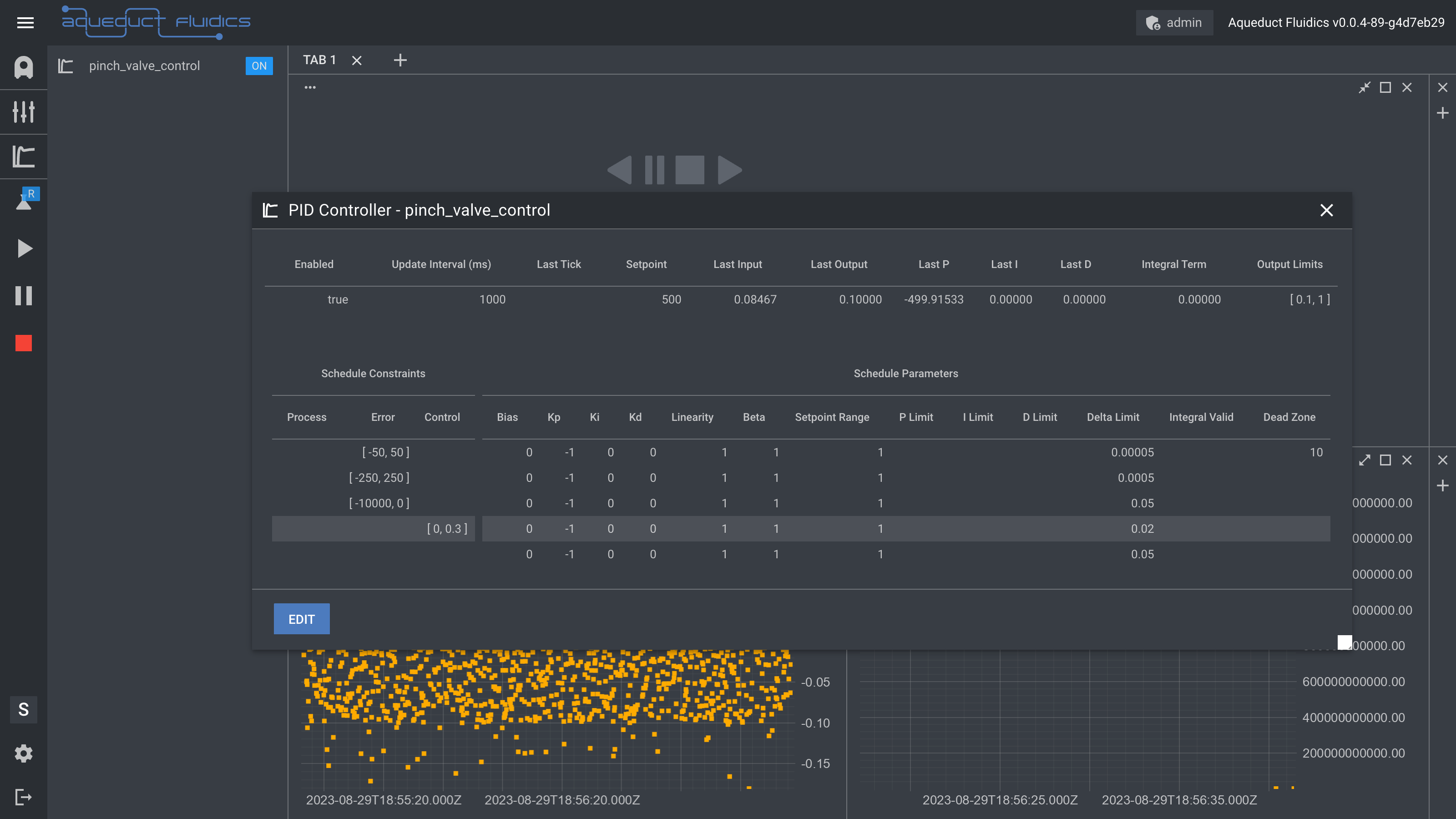
Introduction
The Aqueduct PID Controller API allows you to regulate a device's Control Output by utilizing the value of another device's Process Values. This dynamic control mechanism can be used for:
-
Backpressure Control: Use readings from a pressure transducer as the Process Value to precisely adjust a pinch valve's position as the Control Output. This may be used to control the backpressure within a Tangential Flow Filtration (TFF) system.
-
Weight-based Pump Regulation: Use weight reading from a balance as a Process Value to govern the rate of a peristaltic pump as the Control Output. This may be used to achieve or sustain a target weight, making it ideal for dosing applications.
-
Flow Rate Compensation: Use readings from a mass flow meter as the Process Value to adjust the flow rate of a peristaltic pump as the Control Output. This may be used to compensate for variations between nominal and actual flow rates.
-
pH-based Pump Regulation: Use readings from a pH probe as a Process Value to dynamically adjust the rate of a peristaltic pump as the Control Output. This maintains the desired pH level by controlling the flow of a pH-modifying solution.
Available Process Values and Control Outputs by Device Type
The examples listed above are by no means exhaustive. The API's versatility allows you to design custom control mechanisms by linking any Control Output with any available Process Value from another (or the same) device.
The following table gives an overview of the allowed Process Values and Control Outputs for different device types.
| Device Type | Allowed Process Values | Allowed Control Outputs |
|---|---|---|
| Peristaltic Pump | --- | Flow Rate |
| Syringe Pump | --- | --- |
| Solenoid Valve | --- | --- |
| Rotary Valve | --- | --- |
| Pinch Valve | --- | Position |
| Temperature Probe | Temperature | --- |
| pH Probe | pH | --- |
| Optical Density | Optical Density, Transmitted Intensity, 90° Intensity | --- |
| Mass Flow Meter | Flow Rate | --- |
| Pressure Transducer | Pressure | --- |
| Balance | Weight | --- |
Features
The Aqueduct PID Controller API offers:
-
Schedule-based Parameter Selection:
- Dynamically selects control parameters based on Process Value, Control Output, or Error.
- Useful for managing non-linear processes with different operating regions.
- Example: Pinch valve control in the pinch valve application.
-
Contribution Limiting for P, I, or D Terms:
- Allows limiting the contribution of individual terms to the Control Output.
- Prevents issues like integral windup and excessive derivative action.
- Enhances control stability and performance.
-
Process Value-based Derivative Calculation:
- Utilizes the derivative of the Process Value instead of the derivative of the Error.
- Helps avoid undesirable control actions like derivative kick.
- Improves response to changes in the process variable.
-
Limiting of Maximum \(\Delta CO\) (Change in Control Output):
- Restricts the maximum change in control output between consecutive updates.
- Prevents abrupt and unwanted fluctuations in the control output.
- Example: Capping the maximum change in pinch valve position at 5%.
-
Dead Zone Functionality:
- Configurable band around the setpoint where the controller remains inactive.
- Prevents continuous adjustments within a specific range of the setpoint.
- Example: No adjustments to pump rate when pH is within 0.01 of the setpoint.
-
Control Output Limiting:
- Sets a boundary for the total process control output within a defined range.
- Ensures the control action remains within safe and effective limits.
- Example: Imposing a maximum rate on a peristaltic pump of 5 mL/min.
Overview of PID Control
Proportional-Integral-Derivative (PID) control is a widely used feedback control mechanism that strives to maintain a desired system state by adjusting a control output based on the difference between a setpoint and a measured process value. The Aqueduct PID Controller API provides a toolset for implementing PID control in various applications, offering efficient management of control loops.
Key Components of PID Control
-
Proportional (P) Term: The proportional term produces an output proportional to the current error (difference between setpoint and process value). It acts to bring the system closer to the desired state. Adjusting the proportional gain (kp) amplifies or dampens the response to error, influencing the control output's speed and stability.
-
Integral (I) Term: The integral term considers the cumulative effect of past errors and generates an output to eliminate the accumulated error over time. This is particularly useful in handling steady-state errors and eliminating biases. The integral gain (ki) controls the rate at which the accumulated error is corrected.
-
Derivative (D) Term: The derivative term anticipates the future error trend by evaluating the rate of error change. It provides a damping effect, preventing overshooting and oscillations. The derivative gain (kd) influences the system's responsiveness to rapid changes in error.
PID Controller Algorithm
This guide explains the features of the Aqueduct PID Controller API. It covers the PID Update Process and shows how each user-configurable parameter affects the controller output.
Glossary
| Symbol | Meaning | Detail |
|---|---|---|
| \(SP\) | Setpoint, the target Process Value | in units of \(PV\) |
| \(PV\) | Process Value | |
| \(Error\) | Deviation between Setpoint and Input | \(Error := SP - PV \) |
| \(CO\) | Control Output | |
| \(Δt\) | Time Difference between updates | user configurable update interval, minimum 100 ms |
| \(P\) | Proportional Term | |
| \(I\) | Accumulated Sum of Error * Ki | |
| \(D\) | Derivative Term | |
| \(CO_{\text{min}}\) | Minimum Limit for Control Output | in units of \(CO\) |
| \(CO_{\text{max}}\) | Maximum Limit for Control Output | in units of \(CO\) |
| Schedule Constraints | Meaning | Detail |
|---|---|---|
| \([Error_{\text{min}}, Error_{\text{max}}]\) | Error Range | restrict the schedule to apply when the error falls in the provided range |
| \([PV_{\text{min}}, PV_{\text{max}}]\) | Process Range | restrict the schedule to apply when the process value falls in the provided range |
| \([CO_{\text{min}}, CO_{\text{max}}]\) | Control Range | restrict the schedule to apply when the control output falls in the provided range |
| Schedule Parameters | Meaning | Detail |
|---|---|---|
| \(Bias\) | Bias Offset | |
| \(K_{p}\) | Proportional Gain | positive value direct acting, negative value reverse acting |
| \(K_{i}\) | Integral Gain | positive value direct acting, negative value reverse acting |
| \(K_{d}\) | Derivative Gain | positive value direct acting, negative value reverse acting |
| \(P\) | Proportional Term | |
| \(P_{\text{limit}}\) | Limit for Proportional Term | |
| \(I_{\text{limit}}\) | Limit for Integral Term | |
| \(D_{\text{limit}}\) | Limit for Derivative Term | |
| \(β\) | Setpoint Weighting Factor | |
| \(L\) | Linearity Factor | |
| \(SP_{\text{range}}\) | Setpoint Range | |
| \(DZ\) | Dead Zone | in units of \(PV\) |
| \(I_{\text{valid}}\) | Integral Valid Bounds | in units of \(PV\) |
| \(\Delta CO_{\text{limit}}\) | Maximum Control Output Change | in units of \(CO\) |
Priority-Based Parameter Scheduling
The PID Control Algorithm incorporates the concept of "schedules" into the traditional PID control framework. Each PID controller features a list of schedules, where each schedule is defined by a set of constraints and parameters such as \(K_p\), \(K_i\), \(K_d\), dead zones, and limits.
At each time step, the algorithm evaluates the list of schedules starting from the highest-priority index (index 0). It selects the first schedule whose constraints are met based on real-time data and user-defined conditions. Once a schedule is selected, the PID controller then calculates and updates the Control Output (CO) using the parameters defined in that schedule. This hierarchical and dynamic approach enables the algorithm to adapt to a variety of operating conditions, making it both robust and versatile.
Understanding Controller Schedules
-
Priority Order: The schedules in the list are arranged based on priority, with the highest-priority schedule at the beginning of the list. The schedules cannot be re-ordered after the controller is created.
-
Schedule Constraints: Each schedule is associated with constraints for the process value, error, and control output. These constraints define the range of conditions under which the controller schedule is applicable. If a constraint is left empty, it is considered always applicable.
-
Controller Selection: When the control system receives new process, error, and control values, it starts by checking the controller schedule with the highest priority. It verifies if the current values fall within the defined bounds for that schedule using the
is_applicablemethod. -
Applicability Check: If the current values satisfy the bounds of the constraints, the control system selects that schedule for execution.
-
Fallback and Next Priority: If the highest-priority schedule is not applicable, the control system moves to the next schedule in the list and repeats the applicability check. This process continues until an applicable schedule is found or all schedules have been checked.
Benefits of Controller Scheduling
-
Adaptability: Controller scheduling allows the control system to adapt to varying conditions without manual intervention. Different schedules can be tailored to different operating scenarios.
-
Optimization: By choosing the appropriate schedule, the control system can optimize its performance for specific conditions, leading to improved stability and efficiency.
-
Structured Approach: The priority-based organization of schedules provides a structured way to handle different scenarios, ensuring that the most suitable schedule is chosen.
Controller Selection
At each update tick, the following algorithm is used to determine the applicable schdule:
flowchart TD

A((Start)) --> B[Set i = 0]
B --> C{Is i less\nthan the number\nof schedules?}
C -->|Yes| D{Check\nError\nConstraint}
D -->|Error constraint provided\nand out of bounds bounds| H{Continue}
D -->|Otherwise| F{Check\nProcess\nConstraint}
G --> C
F -->|Process constraint provided\nand out of bounds| H{Continue}
F -->|Otherwise|I{Check\nControl\nConstraint}
H --> G[Increase i by 1]
I --> K((Select\nSchedule i))
I -->|Control constraint provided\nand out of bounds| H{Continue}
C -->|No| J((No Applicable\nSchedule))

click D "#check-error-constraint" _blank
click F "#check-process-constraint" _blank
click I "#check-control-constraint" _blank
Check Error Constraint
If an error constraint is defined for the schedule and the error value falls within the specified range, the schedule is considered applicable with respect to the error constraint. If no error constraint is defined for the current schedule, it is automatically considered applicable for this constraint.
\[ \text{error_is_applicable} = \begin{cases} \text{false} & \text{if } E_{\text{constraint}} \text{ is provided and error not in bounds} \\ \text{true} & \text{otherwise} \end{cases} \]
Check Process Constraint
If a process constraint is defined within the schedule, the algorithm checks to see whether the current process variable (\(PV\)) falls within the specified bounds. If it does, the schedule is considered applicable concerning the process constraint. If no process constraint is defined for the current schedule, then it is automatically considered applicable for this constraint.
\[ \text{process_is_applicable} = \begin{cases} \text{false} & \text{if } PV_{\text{constraint}} \text{ is provided and } PV \text{ not in bounds} \\ \text{true} & \text{otherwise} \end{cases} \]
Check Control Constraint
Similarly, if a control constraint is specified within the schedule, the algorithm evaluates whether the current Control Output (\(CO\)) is within the defined limits. If it is, the schedule is deemed applicable with respect to the control constraint. If no control constraint is specified for the schedule, it is automatically considered applicable for this constraint.
\[ \text{control_is_applicable} = \begin{cases} \text{false} & \text{if } CO_{\text{constraint}} \text{ is provided and } CO \text{ not in bounds} \\ \text{true} & \text{otherwise} \end{cases} \]
Example
Consider the example schedule below:
| Schedules | Error Range | Process Range | Control Range |
|---|---|---|---|
| Schedule 0 | [-50, 50] | [100, 110] | |
| Schedule 1 | [500, 600] | ||
| Schedule 2 |
Example 1:
| Error | Process | Control |
|---|---|---|
| -30 | 550 | 105 |
- Start at Schedule 0:
- Error (-30) is within the range of -50 to 50, so the error constraint is in bounds.
- No Process constraint is provided for Schedule 0, so continue to Control constraint.
- Control (105) is within the range of 100 to 110, so the control constraint is in bounds.
- Schedule 0 is selected and the parameters for Schedule 0 are used to determine the control output.
Example 2:
| Error | Process | Control |
|---|---|---|
| 75 | 590 | 105 |
- Start at Schedule 0:
- Error (75) is not within the range of -50 to 50, so Schedule 0's error constraint is out of bounds.
- Move to Schedule 1:
- No Error constraint is provided for Schedule 1, so continue to Process constraint.
- Process (590) is within the range of 500 to 600, so the process constraint is in bounds.
- No Control constraint is provided for Schedule 1.
- Schedule 1 is selected and the parameters for Schedule 1 are used to determine the control output.
Example 3:
| Error | Process | Control |
|---|---|---|
| -20 | 750 | 720 |
- Start at Schedule 0:
- Error (-20) is within the range of -50 to 50, so the error constraint is in bounds.
- No Process constraint is provided for Schedule 0, so continue to Control constraint.
- Control (720) is not within the range of 100 to 110, so the control constraint is out of bounds.
- Move to Schedule 1:
- No Error constraint is provided for Schedule 1, so continue to Process constraint.
- Process (750) is not within the range of 500 to 600, so Schedule 1's process constraint is out of bounds.
- Move to Schedule 2:
- No bounds are defined for Error, Process, or Control for Schedule 2, so this schedule is applicable by default.
- The parameters for Schedule 2 are used to determine the control output.
Update Process
After a schedule has been selected, the following algorithm is used to determine the control output at time \(t\) based on the schedule's parameters.
flowchart TD

A((Time t)) -->|PV_t, SP_t, L, β, K_p, K_i, K_d, Δt_s, Bias| B(Error_t = SP_t - PV_t)
B -->|Dead Zone Check| C{Error_t < DZ}
C -->|No| F[Calculate Proportional Term]
C -->|Yes| E((No Control Output))
F --> G[Calculate Integral Term]
G --> H[Calculate Derivative Term]
H --> I[Calculate Unbounded Control Output]
I --> J[Limit Control Output Change]
J --> K[Limit Control Output]
K --> L((Control Output at t))

click B "#error-calculation" _blank
click C "#dead-zone-check" _blank
click F "#calculate-proportional-term" _blank
click G "#calculate-integral-term" _blank
click H "#calculate-derivative-term" _blank
click I "#calculate-unbounded-control-output" _blank
click J "#limit-the-control-output-change" _blank
click K "#limit-the-control-output" _blank
Error Calculation
The control output:
\(CO_{t} := \text{control output at time } t \)
based on the process value at time \(t\):
\(PV_{t} := \text{process value at time } t \)
and the user-configurable controller parameters.
The error at time \(t\) is:
\(Error_{t} := \text{error at time } t = SP_{t} - PV_{t} \)
Dead Zone Check
The dead zone is a range around the desired setpoint where no control action is taken. If the absolute value of the error is smaller than the absolute value of the dead zone \(DZ\), no adjustment is made to the Control Output.
\[ |Error_{t}| < |DZ| \Rightarrow \text{no action} \]
Calculate the Proportional Term
Next, the proportional term is calculated using an error term that incorporates the non-linear scalings:
\[ \text{Non-Linear Error} = \left( \beta \times SP_{t} - PV_{t} \right) \times \left( \text{L} + \left( 1 - \text{L} \right) \times \frac{\left| \beta \times SP_{t} - PV_{t} \right|}{SP_{range}} \right) \]
When \( L = 1 \), the non-linear error is equivalent to the linear error.
The proportional term \( P \) is calculated by multiplying the non-linear error by the proportional gain \(K_{p}\), resulting in an unbounded proportional value \( P_{\text{unbounded}} \):
\[ P_{\text{unbounded}} = \text{Non-Linear Error} \times K_p \]
If a limit \( P_{\text{limit}} \) is provided and the unbounded proportional term \( P_{\text{unbounded}} \) is less than the negative value of the limit, then the proportional term \( P \) is set to the negative limit \( -P_{\text{limit}} \). Similarly, if the limit is provided and the unbounded proportional term \( P_{\text{unbounded}} \) exceeds the limit, then the proportional term \( P \) is set to the limit \( P_{\text{limit}} \). Otherwise, if no limit conditions are met, the proportional term \( P \) remains the same as the unbounded value \( P_{\text{unbounded}} \):
\[ P = \begin{cases} -|P_{\text{limit}}| & \text{if } P_{\text{limit}} \text{ is provided and } P_{\text{unbounded}} < -|P_{\text{limit}}| \\ |P_{\text{limit}}| & \text{if } P_{\text{limit}} \text{ is provided and } P_{\text{unbounded}} > |P_{\text{limit}}| \\ P_{\text{unbounded}} & \text{otherwise} \end{cases} \]
Calculate the Integral Term
Next, the integral is checked for validity. If no \(I_{\text{valid}}\) value is provided, the \(\text{valid_integral}\) is considered true. If \(I_{\text{valid}}\) is provided and the absolute value of the error is less than the absolute value of \(I_{\text{valid}}\), then \(\text{valid_integral}\) is also considered true. Otherwise, it is set to false.
\[ \text{valid_integral} = \begin{cases} \text{true} & \text{if } I_{\text{valid}} \text{ is not provided} \\ \text{true} & \text{if } I_{\text{valid}} \text{ is provided and } |\text{error}| < |I_{\text{valid}}| \\ \text{false} & \text{otherwise} \end{cases} \]
The \(I_{\text{unbounded}}\) value is updated based on the \(\text{valid_integral}\) determination.
\[ I_{\text{unbounded}} = \begin{cases} I + \text{error} \times K_{i} \times \Delta t_s & \text{if } \text{valid_integral} \text{ is true} \\ I & \text{otherwise} \end{cases} \]
Finally, the new \(I\) term is calculated based on the provided (\( I_{\text{limit}} \)).
\[ I = \begin{cases} -|I_{\text{limit}}| & \text{if } I_{\text{limit}} \text{ is provided and } I_{\text{unbounded}} < -|I_{\text{limit}}| \\ |I_{\text{limit}}| & \text{if } I_{\text{limit}} \text{ is provided and } I_{\text{unbounded}} > |I_{\text{limit}}| \\ I_{\text{unbounded}} & \text{otherwise} \end{cases} \]
Calculate the Derivative Term
The unbounded derivative term is calculated using:
\[ D_{\text{unbounded}} = -\frac{PV_{t} - PV_{t-1}}{\Delta t_s} \times K_d \]
The new \(D\) term is calculated based on the provided (\( D_{\text{limit}} \)).
\[ D = \begin{cases} -|D_{\text{limit}}| & \text{if } D_{\text{limit}} \text{ is provided and } D_{\text{unbounded}} < -|D_{\text{limit}}| \\ |D_{\text{limit}}| & \text{if } D_{\text{limit}} \text{ is provided and } D_{\text{unbounded}} > |D_{\text{limit}}| \\ D_{\text{unbounded}} & \text{otherwise} \end{cases} \]
Calculate Unbounded Control Output
The unbounded control output is calculated:
\[ CO_{t} = P + I + D + Bias \]
Limit the Control Output Change
The controller allows for limiting sudden changes in the control output \( CO \). The change in the control output between two consecutive time points is calculated:
\[ \Delta CO_{\text{unbounded}} = CO_{t} - CO_{t-1} \]
If \( \Delta CO_{\text{limit}} \) is set and the calculated change is smaller than \( -\Delta CO_{\text{limit}} \), the change is capped at \( -\Delta CO_{\text{limit}} \). If \( \Delta CO_{\text{limit}} \) is set and the change exceeds it, the change is limited to \( \Delta CO_{\text{limit}} \). Otherwise, if the calculated change is within limits, it remains unchanged.
\[ \Delta CO_{t} = \begin{cases} -|\Delta CO_{\text{limit}}| & \text{if } \Delta CO_{\text{limit}} \text{ is provided and } \Delta CO_{\text{unbounded}} < -|\Delta CO_{\text{limit}}| \\ |\Delta CO_{\text{limit}}| & \text{if } \Delta CO_{\text{limit}} \text{ is provided and } \Delta CO_{\text{unbounded}} > |\Delta CO_{\text{limit}}| \\ \Delta CO_{\text{unbounded}} & \text{otherwise} \end{cases} \]
The control output at time \( CO_{t} \) is updated by adding the calculated change \( \Delta CO_{t} \) to the previous output at \( CO_{t-1} \).
\[ CO_{t} = CO_{t-1} + \Delta CO_{\text{t}} \]
Limit the Control Output
Finally, the calculated output is adjusted to ensure that it adheres to any predefined output limits provided by the user:
\[ CO_{t} = \begin{cases} CO_{\text{min}} & \text{if } CO_{\text{min}} \text{ is provided and } CO_{t} < CO_{\text{min}} \\ CO_{\text{max}} & \text{if } CO_{\text{max}} \text{ is provided and } CO_{t} > CO_{\text{min}} \\ CO_{t} & \text{otherwise} \end{cases} \]
Monitoring and Modifying PID Controllers in the Sandbox
Once you create a PID Controller using the Python API, you can monitor real-time data and edit specific parameters in the Sandbox.
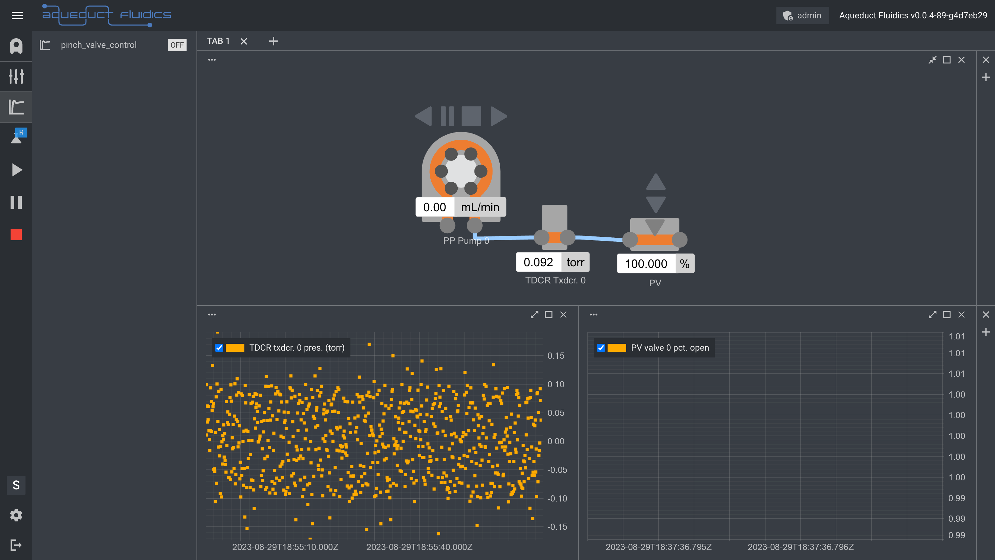
Toggle the PID Controllers menu by pressing the PID Menu Toggle in the left side menu:
| PID Controller Menu Toggle |

|
The menu displays a list of PID Controllers by name, each with an adjacent 'ON/OFF' toggle button.
Use the button to activate or deactivate the controller.
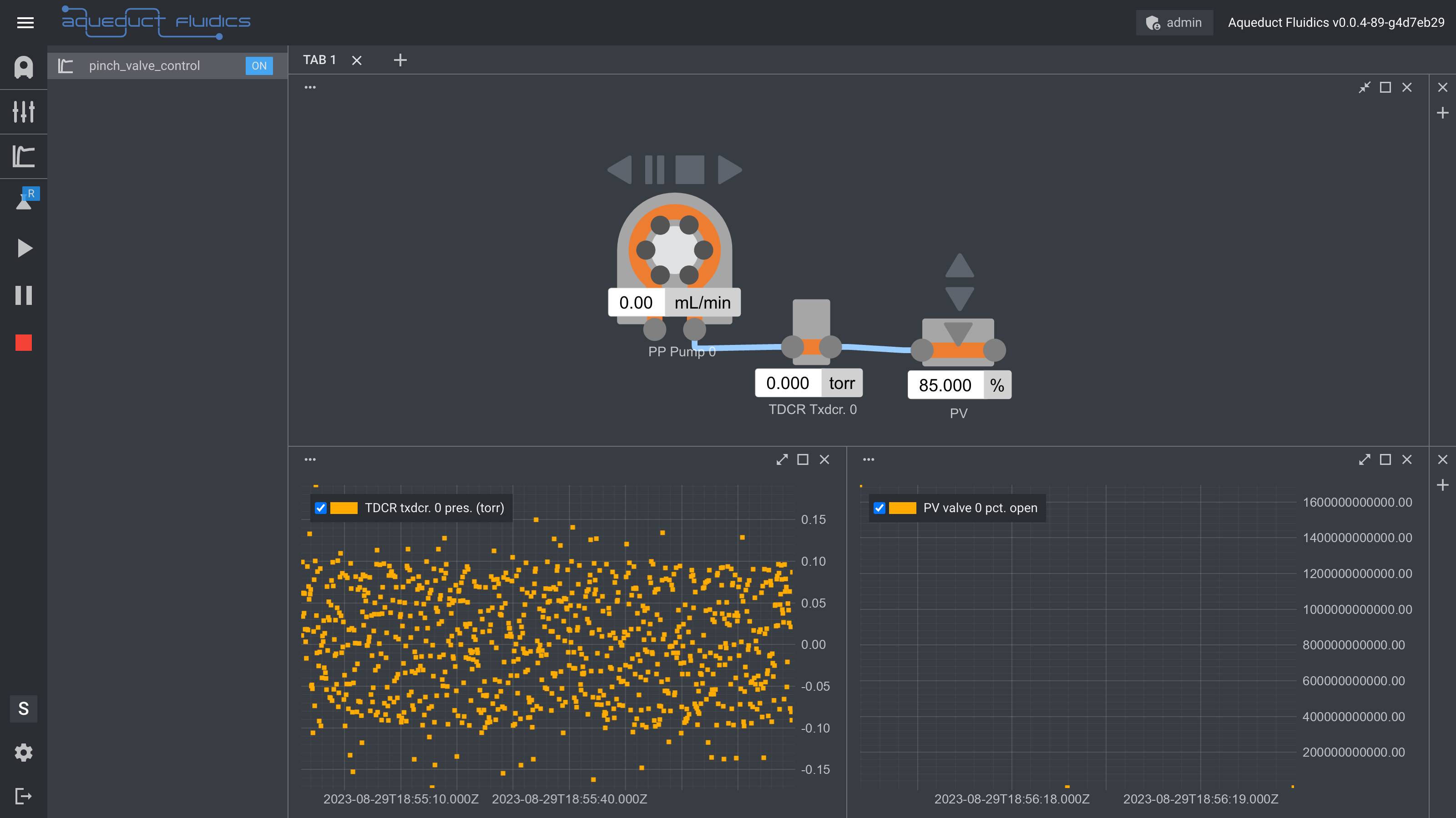
Detailed View
Click on a PID Controller to reveal a table containing detailed information about the current output and schdule list. You can drag the table around the screen using the top of the pop up window and resize the window using the grab handle in the lower right corner.
In the upper row, you'll see a table containing:
-
Enabled: This shows whether the PID Controller is currently active or not. Toggle the active state using the ON/OFF button in the controller side menu.
-
Update Interval (ms): This specifies the time interval in milliseconds at which the PID Controller updates its calculations and output. In Edit Mode, you can modify this value.
-
Setpoint: This is the target value that the PID controller is trying to achieve. In Edit Mode, you can modify this value to change the setpoint.
-
Last Tick: This represents the timestamp of the last update cycle, providing you with a sense of the timing and latency involved in the control loop.
-
Last Input: This displays the last Process Value variable that the PID Controller has read. It is updated at every "tick" defined by the update interval.
-
Last Output: This shows the last Control Output generated by the PID algorithm, giving you immediate feedback on the control action being taken.
-
Last P: This shows the contribution of the Proportional term to the last Control Output.
-
Last I: This shows the contribution of the Integral term to the last Control Output.
-
Last D: This shows the contribution of the Derivative term to the last Control Output.
-
Integral Term: This represents the integral term in the PID algorithm.
-
Output Limits: These are the minimum and maximum values that the PID Controller can output. In Edit Mode, you can modify these values to change the output limits.
In the bottom rows, you'll find a table containing more detailed information about each of the controller's schedules. Each schedule is a row divided into two main sections: Schedule Constraints and Schedule Parameters.
Note: The schedule most recently utilized for computing the Control Output is visually highlighted for quick reference.
Schedule Constraints
-
Process: Lists the acceptable bounds for the Process Variable (PV). If PV is within these bounds, the schedule is applicable with regard to this constraint. In Edit Mode, you can modify this value.
-
Error: Outlines the permissible range for the error value, i.e., the difference between the Setpoint (SP) and the Process Variable (PV). The schedule applies if the error value is within these specified limits. In Edit Mode, you can modify this value.
-
Control: Specifies the allowable Control Output (CO) range. If the CO falls within these limits, the schedule is applicable in terms of the control constraint. In Edit Mode, you can modify this value.
Schedule Parameters
-
Bias: A constant term added to the PID output to facilitate manual fine-tuning or offset compensation. In Edit Mode, you can modify this value.
-
Kp (Proportional Gain): Multiplies the error term, increasing system responsiveness to immediate errors. A higher Kp often leads to quicker error correction but may also induce oscillations. In Edit Mode, you can modify this value.
-
Ki (Integral Gain): Scales the accumulated error term. A higher Ki value accelerates correction for persistent, cumulative errors but risks integral wind-up. In Edit Mode, you can modify this value.
-
Kd (Derivative Gain): Multiplies the rate of change of the error term, effectively 'predicting' future errors. Higher Kd values can prevent overshooting the setpoint but may amplify noise. In Edit Mode, you can modify this value.
-
Linearity: Alters control output behavior in non-linear systems, often useful for dealing with systems whose response varies over its operating range. In Edit Mode, you can modify this value.
-
Beta: Adjusts setpoint weighting to improve performance in systems with notable time delay or inertia. In Edit Mode, you can modify this value.
-
Setpoint Range: Defines a 'success zone' around the setpoint, within which the system is deemed to have adequately achieved its control objective. In Edit Mode, you can modify this value.
-
P Limit: Caps the Proportional term in the PID calculation to prevent excessive control action. In Edit Mode, you can modify this value.
-
I Limit: Sets an upper limit for the Integral term to avoid integral wind-up scenarios, which could otherwise destabilize the system. In Edit Mode, you can modify this value.
-
D Limit: Constrains the Derivative term to prevent it from responding too aggressively to rapid changes or noise in the system. In Edit Mode, you can modify this value.
-
Delta Limit: Specifies the maximum allowable change in Control Output between successive control cycles, enhancing system stability by limiting abrupt control actions. In Edit Mode, you can modify this value.
-
Integral Valid: Demarcates the error range within which the integral term is active, helping to prevent integral wind-up in regions where it might not be beneficial. In Edit Mode, you can modify this value.
-
Dead Zone: Establishes an error range around the setpoint where control actions are intentionally ignored, which minimizes chattering or excessive control activity near the desired value. In Edit Mode, you can modify this value.
Entering Edit Mode
Below the main table, you'll find an "Edit" button. Once clicked, certain cells within the table will change their background color, indicating that these cells are now editable.
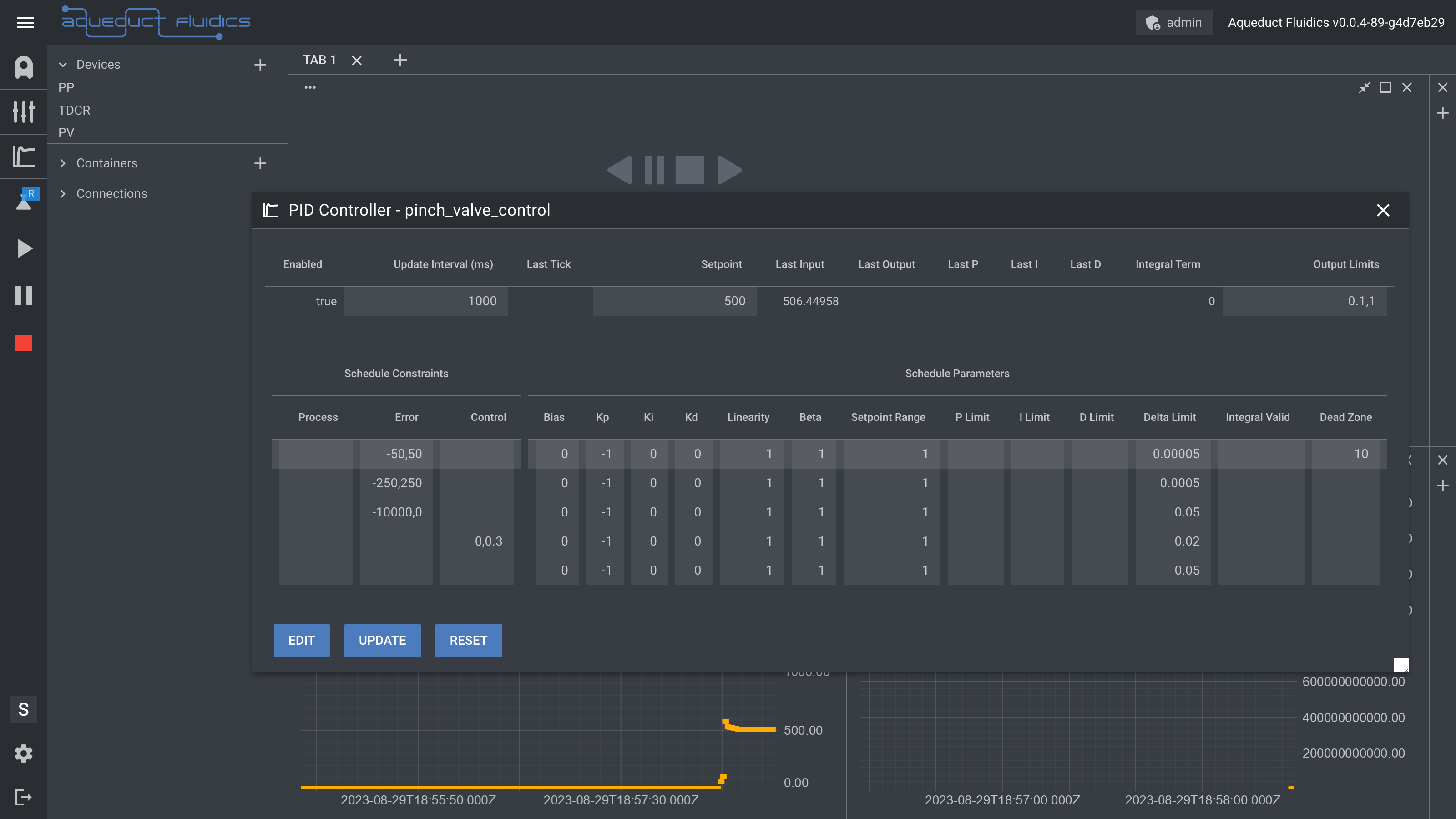
Making Changes
To make a change, simply click on the cell with a different background color and type the new value.
Applying Changes
After editing, click the "Update" button, located at the bottom, to apply your modifications. Click the "Reset" button to revert the values.
Aqueduct PID Controller API Documentation
The Python API allows you to set up PID controllers, change their setpoints, and control their status. You can use the Python API in the context of an Aqueduct Recipe or as a script to create one or more controllers.
Import Required Modules
Start by importing all necessary modules from the Aqueduct library.
Note: The PID API is available on version 0.0.5 and later of
aqueduct-py.
from aqueduct.core.aq import Aqueduct, InitParams
from aqueduct.core.pid import ScheduleParameters, ScheduleConstraints, Pid, Schedule

# your specific device types may differ based on application
from aqueduct.devices.pump.peristaltic import PeristalticPump
from aqueduct.devices.ph import PhProbe
Retrieve Device Instances
Fetch instances of the PeristalticPump and pH Probe devices from the system. We'll use these devices' accessors to create the Process Value and Control Output.
pump: PeristalticPump = aq.devices.get(PUMP_NAME)
ph_probe: PhProbe = aq.devices.get(PH_PROBE_NAME)
Process and Control Value Initialization
After initializing your devices, link them to either a Process Value or a Control Output.
# Generate process and control data for PID controllers.
# Index specifies the node to associate with the accessor.
# (e.g., index=1 would be pH probe node 1)
process_value = ph_probe.to_pid_process_value(index=0)
control_output = pump.to_pid_control_output(index=0)
Create Schedule with Constraints and Parameters
Set up one or more Schedules for the PID controller, including constraints and parameters like kp, ki, kd, etc.
# create a `ScheduleParameters` instance with default values
params = ScheduleParameters()
# change the Bias term
#params.bias = None
# change the Kp term
params.kp = 1
# change the Ki term
params.ki = .025
# change the Kd term
params.kd = .55
# Error values within this range around the setpoint will not activate the controller
params.dead_zone = 0.001
# Integral term will be accumulated when the error is within this limit
params.integral_valid = 0.3
# Change the linearity factor
#params.linearity = 1.0
# Change the beta factor
#params.beta = 1.0
# Change the setpoint range weighting
#params.setpoint_range = 1.0
# Change the limit on the proportional term
#params.p_limit = None
# Change the limit on the integral term
#params.i_limit = None
# Change the limit on the derivative term
#params.d_limit = None
# Change the limit on the maximum change in output
#params.delta_limit = None

constraints = ScheduleConstraints()  # You can add schedule constraints here
# change the process constraints
#constraints.process = (0, 0.35)
# change the error constraints
#constraints.error = (0, 0.35)
# change the control constraints
#constraints.control = (0, 0.35)

# create the schedule
sched = Schedule(params, constraints)
Create PID Instance and Add Schedule
Initialize a PID instance and add the created schedule to it.
p = Pid(8)  # Initialize PID with a setpoint of 8
# Add the schedule to the PID controller
# Since this is the first schedule added, it will
# have the highest priority
p.add_schedule(sched)
Set Output Limits
Define the output limits for the PID controller.
p.output_limits = (0.0, 1) # Output will be constrained within these limits
Create PID Controller Instance
Once you've created your controller, register it with the application using the Aqueduct class's pid_controller method. Here, the name Controller has been assigned to this controller.
pid = aq.pid_controller("Controller", process_value, control_output, p)
Change the Setpoint
Once you've created the controller, you can update the setpoint from the Python API.
pid.change_setpoint(7.5) # Update setpoint to 7.5
Enable or Disable Controller
Control the operational status of the PID controller.
pid.enable()  # Turns the PID controller on
pid.disable()  # Turns the PID controller off
Modify Schedule Parameters
If you want to alter the PID parameters for the first schedule, you can access it via the index from the controllers pid.schedule accessor.
# Update kp to 2 and kd to 0.8 for the first schedule
pid.pid.schedule[0].change_parameters(kp=2, kd=.8)
Complete Code
Here's the complete code from this demo:
from aqueduct.core.aq import Aqueduct, InitParams
from aqueduct.core.pid import ScheduleParameters, ScheduleConstraints, Pid, Schedule

# your specific device types may differ based on application
from aqueduct.devices.pump.peristaltic import PeristalticPump
from aqueduct.devices.ph import PhProbe

# Parse the initialization parameters from the command line
params = InitParams.parse()

# Initialize the Aqueduct instance with the provided parameters
aq = Aqueduct(params.user_id, params.ip_address, params.port)

# Perform system initialization if specified
aq.initialize(params.init)

pump: PeristalticPump = aq.devices.get(PUMP_NAME)
ph_probe: PhProbe = aq.devices.get(PH_PROBE_NAME)

# Generate process and control data for PID controllers.
# Index specifies the node to associate with the accessor.
# (e.g., index=1 would be pH probe node 1)
process_value = ph_probe.to_pid_process_value(index=0)
control_output = pump.to_pid_control_output(index=0)

# create a `ScheduleParameters` instance with default values
params = ScheduleParameters()
# change the Bias term
#params.bias = None
# change the Kp term
params.kp = 1
# change the Ki term
params.ki = .025
# change the Kd term
params.kd = .55
# Error values within this range around the setpoint will not activate the controller
params.dead_zone = 0.001
# Integral term will be accumulated when the error is within this limit
params.integral_valid = 0.3
# Change the linearity factor
#params.linearity = 1.0
# Change the beta factor
#params.beta = 1.0
# Change the setpoint range weighting
#params.setpoint_range = 1.0
# Change the limit on the proportional term
#params.p_limit = None
# Change the limit on the integral term
#params.i_limit = None
# Change the limit on the derivative term
#params.d_limit = None
# Change the limit on the maximum change in output
#params.delta_limit = None

constraints = ScheduleConstraints()  # You can add schedule constraints here
# change the process constraints
#constraints.process = (0, 0.35)
# change the error constraints
#constraints.error = (0, 0.35)
# change the control constraints
#constraints.control = (0, 0.35)

# create the schedule
sched = Schedule(params, constraints)

p = Pid(8)  # Initialize PID with a setpoint of 8
# Add the schedule to the PID controller
# Since this is the first schedule added, it will
# have the highest priority
p.add_schedule(sched)

p.output_limits = (0.0, 1)  # Output will be constrained within these limits

pid = aq.pid_controller("Controller", process_value, control_output, p)
Examples
PID Control for Peristaltic Pump and Balance
- Introduction
- Imports
- Device Configuration
- PID Controller
- PID Control Loop
- Modification of PID Parameters
Introduction
This guide walks you through a sample code that demonstrates how to implement PID control to control the rate of a peristaltic pump based on the weight reading from a balance. The code performs tasks like setting up the devices, configuring PID parameters, and running control loops.
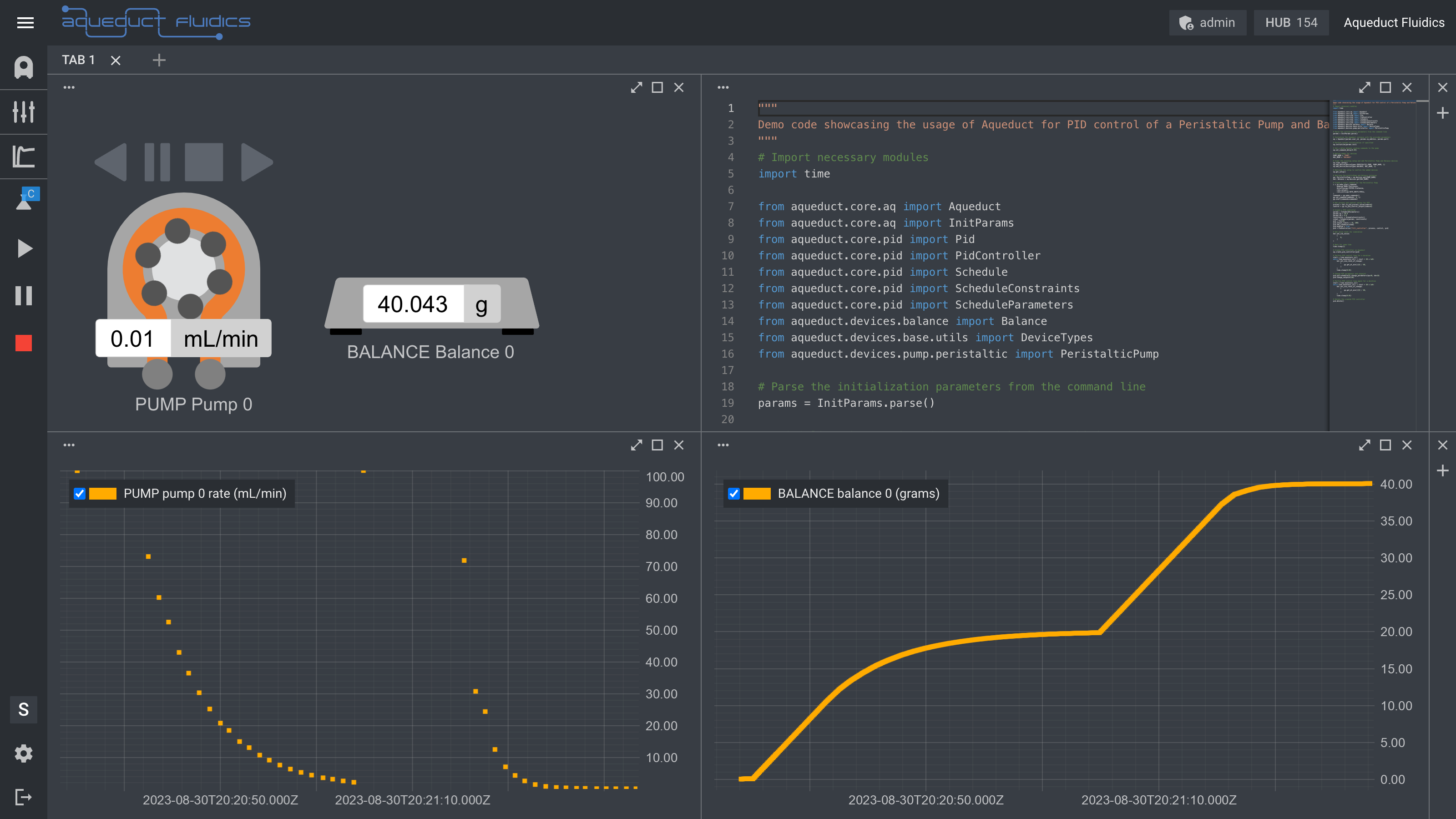
Imports
The first step is to import all the necessary modules from the Aqueduct library.
# Import necessary modules
import time

from aqueduct.core.aq import Aqueduct
from aqueduct.core.aq import InitParams
from aqueduct.core.pid import Pid
from aqueduct.core.pid import PidController
from aqueduct.core.pid import Schedule
from aqueduct.core.pid import ScheduleConstraints
from aqueduct.core.pid import ScheduleParameters
from aqueduct.devices.balance import Balance
from aqueduct.devices.base.utils import DeviceTypes
from aqueduct.devices.pump.peristaltic import PeristalticPump
Initialization
Here, initialization parameters are parsed from the command line and used to initialize the Aqueduct instance.
# Parse the initialization parameters from the command line
params = InitParams.parse()

# Initialize the Aqueduct instance with the provided parameters
aq = Aqueduct(params.user_id, params.ip_address, params.port)
Device Configuration
Clear Setup
Any existing setup should be cleared before adding new devices.
# Clear the existing setup
aq.clear_setup()
Add Devices
This section adds a peristaltic pump and a balance to the setup and then retrieves the newly added devices.
# Add Peristaltic Pump and Balance devices
aq.add_device(DeviceTypes.PERISTALTIC_PUMP, PUMP_NAME, 1)
aq.add_device(DeviceTypes.BALANCE, BAL_NAME, 1)

# Retrieve the setup to confirm the added devices
aq.get_setup()

# Retrieve PeristalticPump and Balance instances
pp: PeristalticPump = aq.devices.get(PUMP_NAME)
bal: Balance = aq.devices.get(BAL_NAME)
PID Controller
PID Parameters and Schedule
Define the PID schedule parameters and constraints. Each PID controller can have multiple schedules. Constraints help to determine which schedule is used at each time step.
# Create a PID controller
params = ScheduleParameters()
params.kp = 10.0
params.kd = 5.0
constraints = ScheduleConstraints()
sched = Schedule(params, constraints)
Creating the PID Controller
The PID controller is then created with the defined schedules.
# Get process and control values for PID
process = bal.to_pid_process_value(index=0)
control = pp.to_pid_control_output(index=0)

pid = PidController("fill_controller", process, control, pid)
PID Control Loop
The code then runs a PID control loop to control the device for a duration.
# Perform PID control loop for a duration
start = time.monotonic_ns()
while time.monotonic_ns() < start + 30 * 1e9:
   # set the sim rate of change of the balance based on the pump rate
   bal.set_sim_rates_of_change(
      [
            pp.get_ml_min()[0] / 60,
      ]
   )
   time.sleep(0.01)
Modification of PID Parameters
Finally, the code shows how to modify PID parameters and rerun the control loop.
# Change PID parameters and setpoint
pid.pid.schedule[0].change_parameters(kp=30, kd=10)
pid.change_setpoint(40)
Here's the full code:
"""
Demo code showcasing the usage of Aqueduct for PID control of a Peristaltic Pump and Balance.
"""
# Import necessary modules
import time

from aqueduct.core.aq import Aqueduct
from aqueduct.core.aq import InitParams
from aqueduct.core.pid import Pid
from aqueduct.core.pid import PidController
from aqueduct.core.pid import Schedule
from aqueduct.core.pid import ScheduleConstraints
from aqueduct.core.pid import ScheduleParameters
from aqueduct.devices.balance import Balance
from aqueduct.devices.base.utils import DeviceTypes
from aqueduct.devices.pump.peristaltic import PeristalticPump

# Parse the initialization parameters from the command line
params = InitParams.parse()

# Initialize the Aqueduct instance with the provided parameters
aq = Aqueduct(params.user_id, params.ip_address, params.port)

# Perform system initialization if specified
aq.initialize(params.init)

# Set a delay between sending commands to the pump
aq.set_command_delay(0.05)

# Define names for devices
PUMP_NAME = "PUMP"
BAL_NAME = "BALANCE"

# Clear the existing setup and add Peristaltic Pump and Balance devices
aq.clear_setup()
aq.add_device(DeviceTypes.PERISTALTIC_PUMP, PUMP_NAME, 1)
aq.add_device(DeviceTypes.BALANCE, BAL_NAME, 1)

# Retrieve the setup to confirm the added devices
aq.get_setup()

# Retrieve PeristalticPump and Balance instances
pp: PeristalticPump = aq.devices.get(PUMP_NAME)
bal: Balance = aq.devices.get(BAL_NAME)

# Create a start command for the Peristaltic Pump
c = pp.make_start_command(
    mode=pp.MODE.Continuous,
    direction=pp.STATUS.Clockwise,
    rate_value=1,
    rate_units=pp.RATE_UNITS.MlMin,
)
commands = pp.make_commands()
pp.set_command(commands, 0, c)
pp.start(commands=commands)

# Get process and control values for PID
process = bal.to_pid_process_value(index=0)
control = pp.to_pid_control_output(index=0)

# Create a PID controller
params = ScheduleParameters()
params.kp = 10.0
params.kd = 5.0
constraints = ScheduleConstraints()
sched = Schedule(params, constraints)
pid = Pid(20)
pid.output_limits = (0, 100)
pid.add_schedule(sched)
pid.enabled = True
pid = PidController("fill_controller", process, control, pid)

# Set noise level for simulation
bal.set_sim_noise(
    [
        0,
    ]
)

# Wait for some time
time.sleep(1)

# Create PID controller on Aqueduct
aq.create_pid_controller(pid)

# Perform PID control loop for a duration
start = time.monotonic_ns()
while time.monotonic_ns() < start + 30 * 1e9:
    bal.set_sim_rates_of_change(
        [
            pp.get_ml_min()[0] / 60,
        ]
    )
    time.sleep(0.01)

# Change PID parameters and setpoint
pid.pid.schedule[0].change_parameters(kp=30, kd=10)
pid.change_setpoint(40)

# Perform PID control loop again for a duration
start = time.monotonic_ns()
while time.monotonic_ns() < start + 30 * 1e9:
    bal.set_sim_rates_of_change(
        [
            pp.get_ml_min()[0] / 60,
        ]
    )
    time.sleep(0.01)

# Delete the created PID controller
pid.delete()
Simulating a Chemical Reaction System with Time-Delayed Response
- Overview
- Running the Scripts
- Code Example 1: Simulating a Chemical Reaction System
- Code Example 2: PID Controller for Multiple Pumps and pH Probes
Overview
This script models a chemical reaction whose pH decreases with time (becomes more acidic) with a rate that also decreases with time (slowing kinetics). The system's pH level increases in response to the addition of a base at a specified rate (mL/min). The model is designed to emulate scenarios with extended time constants, which can present control challenges. Adjustments to the PID controllers are made to effectively manage this time-delayed response.
The intent of the simulated model is to reflect the time-dependent response of the chemical system to the addition of a base, particularly focusing on the system's time constant. The time constant is a critical parameter that characterizes how quickly the system reaches a new steady-state following a perturbation, such as the addition of a base. In this model, we implement the time constant to reflect the delayed impact of the base addition on the system's pH level. This is particularly useful for understanding control challenges associated with systems that have inherent time delays or slow response times. The time constant is integrated into the differential equations governing the rate of change in pH, allowing for a more realistic simulation. Detailed implementation of this concept is provided in the subsequent code sections.
Running the Scripts
To successfully run the simulation and control the system, two separate Python scripts must be executed in a sequential manner.
-
Chemical Reaction Simulation (
model.py): First, initiate the simulation by running themodel.pyscript. Execute the following command in your terminal:python3 examples/pid/ph/model.py -r 0The
-r 0flag ensures that the script does not register as a recipe in the Aqueduct system. -
PID Control (
pid.py): Once the simulation model is up and running, you can launch the PID control script in interactive mode. Use the following command:python3 -i examples/pid/pinch_valve/pid.pyThe
-iflag allows you to interact with the script in real-time after it's been executed, permitting on-the-fly adjustments and queries.
Note: It is essential to start model.py before pid.py to ensure that the simulation environment is properly initialized for the PID control.
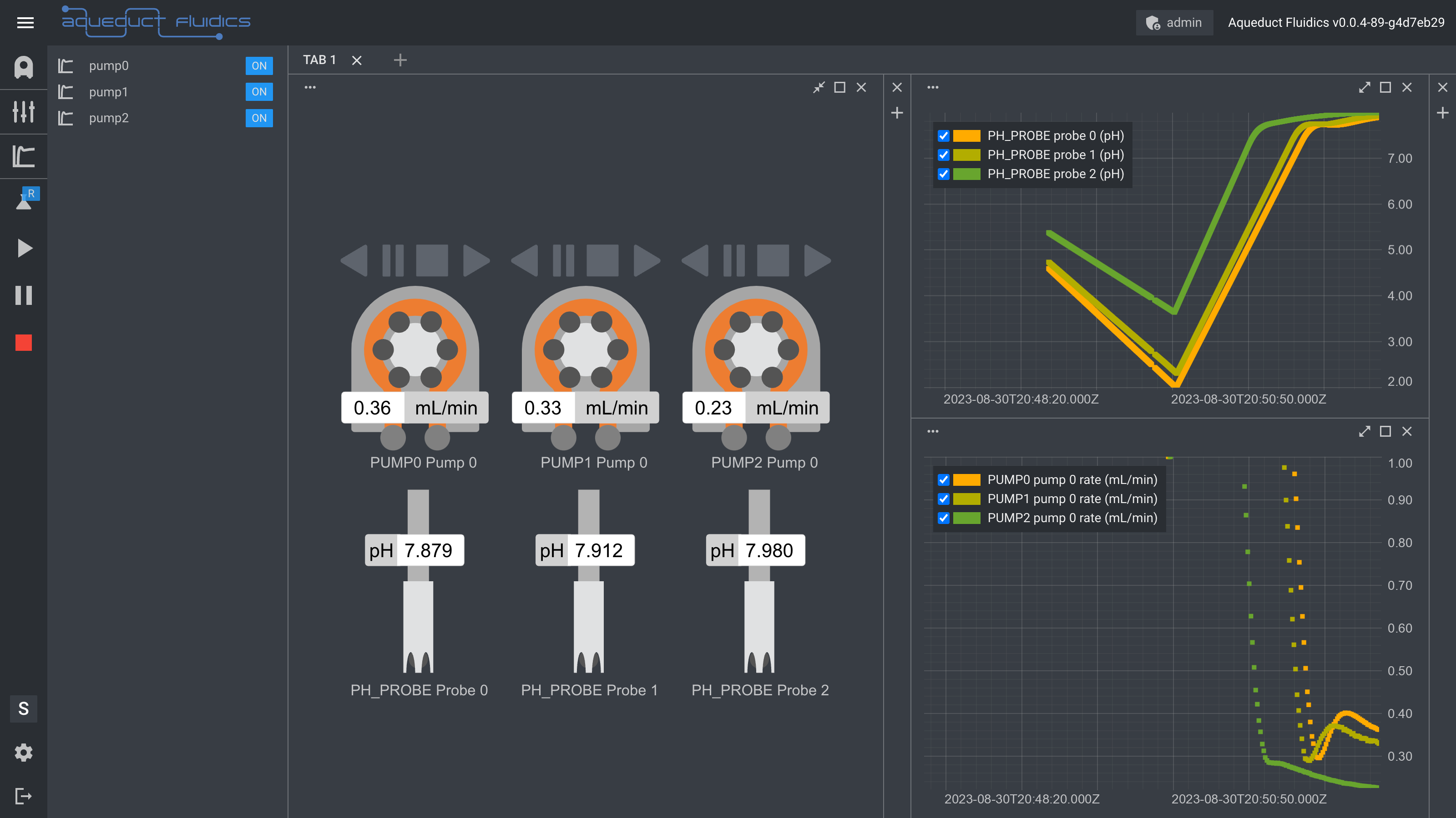
Imports
Import standard Python libraries.
import time
import typing
import random
import threading
Reaction Class
The Reaction class simulates a chemical reaction characterized by varying parameters such as the time constant.
class Reaction:
    def __init__(self):
        """Initialize reaction parameters."""
        self.time_constant_s = round(random.uniform(2, 6), 3)
        # ...
Model Class
Manage multiple Reaction instances and connect them to physical devices like pumps and pH probes.
class Model:
    def __init__(self, pumps: typing.List[PeristalticPump], probe: PhProbe):
        """Initialize the model."""
        self.pumps = pumps
        self.ph_probe = probe
        # ...

    def calculate(self):
        """Calculate rate of pH change."""
        # ...
Here's the full code for the model:
"""
Description: This script models a chemical reaction system using threads for parallel calculations.
It simulates the delay in the response of pH with respect to the change in dose rate, thereby
modeling a time constant in the system.
"""
import argparse
import random
import threading
import time
import typing

from aqueduct.core.aq import Aqueduct
from aqueduct.core.aq import InitParams
from aqueduct.devices.base.utils import DeviceTypes
from aqueduct.devices.ph import PhProbe
from aqueduct.devices.pump.peristaltic import PeristalticPump


class Reaction:
    """
    Models a single chemical reaction by defining parameters to capture
    the rate of change of pH as a function of dose rate (mL/min).

    Attributes:
        reaction_start_time: Time when the reaction started.
        dpH_s_dmL_min_start: Initial slope of pH change per mL/min rate.
        delta_change_s: Change in slope of pH change per second.
        delta_change_bounds: Maximum and minimum rate of change.
        roc_offset: Initial offset of the rate of change.
        last_roc: Last calculated rate of change.
        time_constant_s: Time constant to model delay in pH response.
    """

    def __init__(self):
        """Initialize reaction parameters."""
        self.time_constant_s = round(random.uniform(2, 6), 3)
        self.roc_offset = round(random.uniform(-1.95 / 60, -0.95 / 60), 4)
        self.reaction_start_time: float = None

        self.dpH_s_dmL_min_start: float = 0.095  # (pH/s)/(mL/min)
        self.delta_change_s: float = 0.000005  # (pH/s)/(mL/min*s)
        self.delta_change_bounds: tuple = (-0.5, 0.5)

        self.last_roc = None

    def start_reaction(self) -> None:
        """Record the starting time of the reaction."""
        self.reaction_start_time = time.time()

    def calc_rate_of_change(self, ml_min):
        """
        Calculate the rate of change of pH with respect to the dose rate (mL/min).

        Args:
            ml_min: The dosing rate in mL/min.
        """
        # Calculate the time since the reaction started
        reaction_duration_s = time.time() - self.reaction_start_time

        # Calculate rate of change (roc)
        roc = (
            self.roc_offset
            + (self.dpH_s_dmL_min_start + reaction_duration_s * self.delta_change_s)
            * ml_min
        )

        # Constrain roc within bounds
        roc = max(min(roc, self.delta_change_bounds[1]), self.delta_change_bounds[0])
        roc = round(roc, 4)
        self.last_roc = roc


class Model:
    """
    Main class to manage multiple Reactions and link them with physical devices.

    Attributes:
        reactions: List of Reaction objects.
        delayed_roc: List of delayed rate of change values.
        pumps: List of PeristalticPump objects.
        ph_probe: PhProbe object.
        lock: Threading lock to control concurrent access to shared resources.
    """

    def __init__(self, pumps: typing.List[PeristalticPump], probe: PhProbe):
        """Initialize the model."""
        self.pumps = pumps
        self.ph_probe = probe
        self.reactions = [None] * self.ph_probe.len
        self.lock = threading.Lock()

        for i in range(self.ph_probe.len):
            self.reactions[i] = Reaction()
            self.reactions[i].start_reaction()

    def calculate(self):
        """
        Calculate the rate of change in pH for each reaction and
        update the pH probe simulation.
        """
        rates = [p.live[0].ml_min for p in self.pumps]

        def target(i, m):
            """Target function for threading."""
            time.sleep(m.time_constant_s)
            with self.lock:  # Acquire the lock before updating shared data
                m.calc_rate_of_change(rates[i])

        threads = []
        for (i, m) in enumerate(self.reactions):
            t = threading.Thread(target=target, args=(i, m), daemon=True)
            threads.append(t)
            t.start()

        with self.lock:  # Acquire the lock before updating shared data
            self.ph_probe.set_sim_rates_of_change([r.last_roc for r in self.reactions])


if __name__ == "__main__":

    # Parse the initialization parameters from the command line
    params = InitParams.parse()

    # Initialize the Aqueduct instance with the provided parameters
    aq = Aqueduct(
        params.user_id,
        params.ip_address,
        params.port,
        register_process=params.register_process,
    )

    # Perform system initialization if specified
    aq.initialize(params.init)

    # Set a delay between sending commands to the pump
    aq.set_command_delay(0.05)

    parser = argparse.ArgumentParser()

    parser.add_argument(
        "-c",
        "--clear",
        type=int,
        help="clear and create the setup (either 0 or 1)",
        default=1,
    )

    args, _ = parser.parse_known_args()
    clear = bool(args.clear)

    # Define names for devices
    PUMP0_NAME = "PUMP0"
    PUMP1_NAME = "PUMP1"
    PUMP2_NAME = "PUMP2"
    PH_PROBE_NAME = "PH_PROBE"

    if clear:
        # Clear the existing setup and add devices
        aq.clear_setup()

        aq.add_device(DeviceTypes.PERISTALTIC_PUMP, PUMP0_NAME, 1)
        aq.add_device(DeviceTypes.PERISTALTIC_PUMP, PUMP1_NAME, 1)
        aq.add_device(DeviceTypes.PERISTALTIC_PUMP, PUMP2_NAME, 1)
        aq.add_device(DeviceTypes.PH_PROBE, PH_PROBE_NAME, 3)

    # Retrieve the setup to confirm the added devices
    aq.get_setup()

    # Retrieve device instances
    pump0: PeristalticPump = aq.devices.get(PUMP0_NAME)
    pump1: PeristalticPump = aq.devices.get(PUMP1_NAME)
    pump2: PeristalticPump = aq.devices.get(PUMP2_NAME)
    ph_probe: PhProbe = aq.devices.get(PH_PROBE_NAME)

    ph_probe.set_sim_noise([0.0001, 0.0005, 0.0001])
    ph_probe.set_sim_rates_of_change([-0.1, -0.1, -0.1])

    # Create an instance of the PressureModel
    model = Model([pump0, pump1, pump2], ph_probe)

    # Continuous pressure calculation loop
    while True:
        model.calculate()
        time.sleep(0.5)
PID Control for Multiple Pumps and pH Probes
This script illustrates the setup of PID controllers to govern pump behavior based on pH measurements, enabling precise control of complex systems.
Initialization and Device Setup
Initialize the Aqueduct instance and retrieve device instances.
params = InitParams.parse()
aq = Aqueduct(params.user_id, params.ip_address, params.port)
# Retrieve device instances
pump0: PeristalticPump = aq.devices.get(PUMP0_NAME)
PID Controllers Setup
Configure PID controllers for each pump, using pH measurements as the process value.
controllers = []
for (i, pump) in enumerate([pump0, pump1, pump2]):
    process = ph_probe.to_pid_process_value(index=i)
    # ...
    p = Pid(8)
    p.add_schedule(sched)
Here's the full code for PID control:
"""
Demonstration of setting up a PID controller with Aqueduct devices.
"""
# Import necessary modules
from aqueduct.core.aq import Aqueduct
from aqueduct.core.aq import InitParams
from aqueduct.core.pid import Pid
from aqueduct.core.pid import Schedule
from aqueduct.core.pid import ScheduleConstraints
from aqueduct.core.pid import ScheduleParameters
from aqueduct.devices.ph import PhProbe
from aqueduct.devices.pump.peristaltic import PeristalticPump

# Parse the initialization parameters from the command line
params = InitParams.parse()

# Initialize the Aqueduct instance with the provided parameters
aq = Aqueduct(params.user_id, params.ip_address, params.port)

# Perform system initialization if specified
aq.initialize(params.init)

# Set a delay between sending commands to the pump
aq.set_command_delay(0.05)

# Define names for devices
PUMP0_NAME = "PUMP0"
PUMP1_NAME = "PUMP1"
PUMP2_NAME = "PUMP2"
PH_PROBE_NAME = "PH_PROBE"

# Retrieve the setup to confirm the added devices
aq.get_setup()

# Retrieve device instances
pump0: PeristalticPump = aq.devices.get(PUMP0_NAME)
pump1: PeristalticPump = aq.devices.get(PUMP1_NAME)
pump2: PeristalticPump = aq.devices.get(PUMP2_NAME)
ph_probe: PhProbe = aq.devices.get(PH_PROBE_NAME)

controllers = []

for (i, pump) in enumerate([pump0, pump1, pump2]):
    # Define PID controller parameters
    process = ph_probe.to_pid_process_value(index=i)
    control = pump.to_pid_control_output(index=0)
    p = Pid(8)

    # Define multiple schedules with different controller settings
    for integral_valid, dead_zone in [
        (0.3, 0.0005),
    ]:
        params = ScheduleParameters()
        params.kp = 1
        params.ki = 0.025
        params.kd = 0.55
        params.dead_zone = dead_zone
        params.integral_valid = integral_valid
        constraints = ScheduleConstraints()
        sched = Schedule(params, constraints)
        p.add_schedule(sched)

    # Set output limits for the PID controller
    p.output_limits = (0.0, 1)

    # Create a PID controller instance using Aqueduct
    pid = aq.pid_controller(f"pump{i}", process, control, p)
    controllers.append(pid)
These scripts leverage the Aqueduct library for device management and PID control, offering a comprehensive yet adaptable solution for controlling complex chemical systems.
Pressure Control Using a Pinch Valve: Non-Linear Control Output
- Overview
- Running the Scripts
- Code Example 1: Pressure Model Simulation
- Code Example 2: Complex PID Controller for the Pinch Valve
Overview
This guide aims to demonstrate how to implement a pressure control system using a Pinch Valve. The complexity lies in the unique characteristics of a Pinch Valve, which squeezes an elastomeric tube to regulate back pressure. The valve's flow coefficient (Cv) varies in a non-linear fashion with the valve's plunger position (percentage of travel, from full close to full open). This adds an extra layer of complexity to the control system.
As the valve pinches the tube, the effective opening size and shape change non-linearly. Consequently, the Cv (valve flow coefficient) also changes non-linearly with the percentage of valve opening.
Addressing Non-Linearity through Complex PID Scheduling
To manage this non-linearity, the controller must be designed to operate differently in various regions of operation. Specifically, when the total percentage of the valve's opening is small, the maximum control output change (delta_limit) has to be very small to avoid overshooting or other adverse effects.
The PID controller code includes a scheduling system that changes the control parameters based on the operating conditions. Here's a snippet of that part:
# Define multiple schedules with different controller settings
for error_range, control_range, delta_limit, dead_zone in [
    ((-50, 50), None, 0.00005, 10),
    ((-250, 250), None, 0.0005, None),
    ((-10000, 0), None, 0.05, None),
    (None, (0, 0.3), 0.020, None),
    (None, None, 0.050, None),
]:
    params = ScheduleParameters()
    params.kp = -1.0
    params.dead_zone = dead_zone
    params.delta_limit = delta_limit
    constraints = ScheduleConstraints()
    constraints.error = error_range
    constraints.control = control_range
    sched = Schedule(params, constraints)
    p.add_schedule(sched)
This scheduling system allows the controller to operate with different settings, including a dead zone, delta limits, and control ranges, depending on the state of the system. This makes it adaptable and more accurate, particularly when dealing with the non-linear characteristics of the Pinch Valve.
Running the Scripts
To run the simulation and control, you'll need to execute two separate Python scripts in sequence:
-
Pressure Model Simulation (
model.py): First, run themodel.pyscript to simulate the pressure control system. Execute this command in your terminal:python3 examples/pid/pinch_valve/model.py -r 0 -
Complex PID Controller (
pid.py): Oncemodel.pyis running, execute thepid.pyscript. This will set up a PID controller to regulate the Pinch Valve based on the pressure readings. Run this command:python3 -i examples/pid/pinch_valve/pid.py
Note: It's crucial to run model.py before executing pid.py to ensure the simulation environment is initialized correctly.
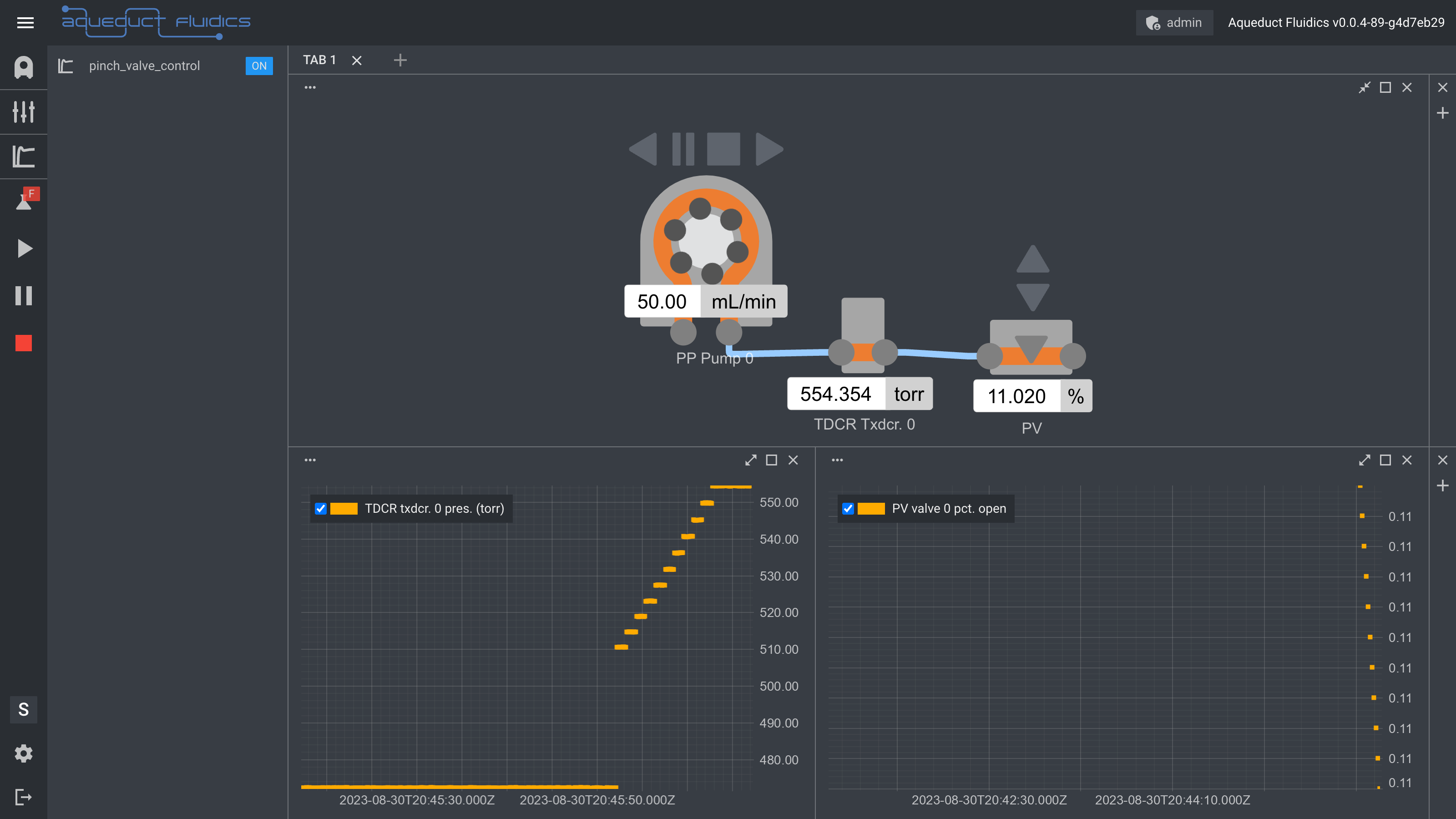
Code Example 1: Pressure Model Simulation
Imports
import argparse
import time
from aqueduct.core.aq import Aqueduct
from aqueduct.core.aq import InitParams
from aqueduct.devices.base.utils import DeviceTypes
from aqueduct.devices.pressure.transducer import PressureTransducer
from aqueduct.devices.pressure.transducer import PressureUnits
from aqueduct.devices.pump.peristaltic import PeristalticPump
from aqueduct.devices.valve.pinch import PinchValve
The PressureModel Class
The PressureModel class simulates a pressure control system using various devices such as a pump, pinch valve, and pressure transducer.
class PressureModel:
    def __init__(self, pump: PeristalticPump, pinch_valve: PinchValve, transducer: PressureTransducer, aqueduct: "Aqueduct"):
        self.pump = pump
        self.pv = pinch_valve
        self.tdcr = transducer
        self.aq = aqueduct
    # ...
Here's the full code for the model:
"""
Demo code demonstrating pressure estimation using a simple model for Aqueduct devices.
"""
# Import necessary modules
import argparse
import time

from aqueduct.core.aq import Aqueduct
from aqueduct.core.aq import InitParams
from aqueduct.devices.base.utils import DeviceTypes
from aqueduct.devices.pressure.transducer import PressureTransducer
from aqueduct.devices.pressure.transducer import PressureUnits
from aqueduct.devices.pump.peristaltic import PeristalticPump
from aqueduct.devices.valve.pinch import PinchValve


class PressureModel:
    """
    Simple model for estimating pressures in a filtration process using Aqueduct devices.
    """

    filtration_start_time: float = None
    filter_cv_retentate: float = 60

    def __init__(
        self,
        pump: PeristalticPump,
        pinch_valve: PinchValve,
        transducer: PressureTransducer,
        aqueduct: "Aqueduct",
    ):
        self.pump = pump
        self.pv = pinch_valve
        self.tdcr = transducer
        self.aq = aqueduct

    @staticmethod
    def calc_pv_cv(PV) -> float:
        """
        Calculate the Cv of the pinch valve.

        :param PV: Pinch valve position.
        :type PV: float

        :return: Cv of the pinch valve.
        :rtype: float
        """
        if PV < 0.35:
            return max(100 - (1 / PV**2), 1)
        else:
            return 100

    def calc_p1(self, R1, PV) -> float:
        """
        Calculate the pressure drop between retentate and permeate.

        :param R1: Flow rate in the pass-through leg of the TFF filter.
        :type R1: float

        :param PV: Pinch valve position.
        :type PV: float

        :return: Pressure drop between retentate and permeate.
        :rtype: float
        """
        try:
            return 1 / (PressureModel.calc_pv_cv(PV) * 0.865 / R1) ** 2
        except ZeroDivisionError:
            return 0

    def calc_pressures(self):
        """
        Calculate and update the pressures using the model equations.
        """
        p1 = self.calc_p1(self.pump.live[0].ml_min, self.pv.live[0].pct_open)
        p1 = min(p1, 50)
        self.tdcr.set_sim_values(values=(p1,), units=PressureUnits.PSI)


if __name__ == "__main__":

    # Parse the initialization parameters from the command line
    params = InitParams.parse()

    # Initialize the Aqueduct instance with the provided parameters
    aq = Aqueduct(
        params.user_id,
        params.ip_address,
        params.port,
        register_process=params.register_process,
    )

    # Perform system initialization if specified
    aq.initialize(params.init)

    # Set a delay between sending commands to the pump
    aq.set_command_delay(0.05)

    parser = argparse.ArgumentParser()

    parser.add_argument(
        "-c",
        "--clear",
        type=int,
        help="clear and create the setup (either 0 or 1)",
        default=1,
    )

    args, _ = parser.parse_known_args()
    clear = bool(args.clear)

    # Define names for devices
    PUMP_NAME = "PP"
    XDCR_NAME = "TDCR"
    PV_NAME = "PV"

    if clear:
        # Clear the existing setup and add devices
        aq.clear_setup()

        aq.add_device(DeviceTypes.PERISTALTIC_PUMP, PUMP_NAME, 1)
        aq.add_device(DeviceTypes.PRESSURE_TRANSDUCER, XDCR_NAME, 1)
        aq.add_device(DeviceTypes.PINCH_VALVE, PV_NAME, 1)

    # Retrieve the setup to confirm the added devices
    aq.get_setup()

    # Retrieve device instances
    pp: PeristalticPump = aq.devices.get(PUMP_NAME)
    tdcr: PressureTransducer = aq.devices.get(XDCR_NAME)
    pv: PinchValve = aq.devices.get(PV_NAME)

    # Create an instance of the PressureModel
    model = PressureModel(pp, pv, tdcr, aq)

    # Continuous pressure calculation loop
    while True:
        model.calc_pressures()
        time.sleep(0.1)
Code Example 2: Complex PID Controller for the Pinch Valve
Imports
from aqueduct.core.aq import Aqueduct
from aqueduct.core.aq import InitParams
from aqueduct.core.pid import Pid
from aqueduct.core.pid import Schedule
from aqueduct.core.pid import ScheduleConstraints
from aqueduct.core.pid import ScheduleParameters
from aqueduct.devices.pressure.transducer import PressureTransducer
from aqueduct.devices.pump.peristaltic import PeristalticPump
from aqueduct.devices.valve.pinch import PinchValve
Device Retrieval
pp: PeristalticPump = aq.devices.get(PUMP_NAME)
tdcr: PressureTransducer = aq.devices.get(XDCR_NAME)
pv: PinchValve = aq.devices.get(PV_NAME)
PID Controller Setup
The PID controller is set up with multiple schedules to adapt to the system's non-linear nature.
# Define PID controller parameters
process = tdcr.to_pid_process_value(index=0)
control = pv.to_pid_control_output(index=0)
p = Pid(500)
Here's the full code for PID control:
"""
Demonstration of setting up a PID controller with Aqueduct devices.
"""
# Import necessary modules
from aqueduct.core.aq import Aqueduct
from aqueduct.core.aq import InitParams
from aqueduct.core.pid import Pid
from aqueduct.core.pid import Schedule
from aqueduct.core.pid import ScheduleConstraints
from aqueduct.core.pid import ScheduleParameters
from aqueduct.devices.pressure.transducer import PressureTransducer
from aqueduct.devices.pump.peristaltic import PeristalticPump
from aqueduct.devices.valve.pinch import PinchValve

# Parse the initialization parameters from the command line
params = InitParams.parse()

# Initialize the Aqueduct instance with the provided parameters
aq = Aqueduct(params.user_id, params.ip_address, params.port)

# Perform system initialization if specified
aq.initialize(params.init)

# Set a delay between sending commands to the pump
aq.set_command_delay(0.05)

# Define names for devices
PUMP_NAME = "PP"
XDCR_NAME = "TDCR"
PV_NAME = "PV"

# Retrieve the setup to confirm the added devices
aq.get_setup()

# Retrieve device instances
pp: PeristalticPump = aq.devices.get(PUMP_NAME)
tdcr: PressureTransducer = aq.devices.get(XDCR_NAME)
pv: PinchValve = aq.devices.get(PV_NAME)

# Define PID controller parameters
process = tdcr.to_pid_process_value(index=0)
control = pv.to_pid_control_output(index=0)
p = Pid(500)

# Define multiple schedules with different controller settings
for error_range, control_range, delta_limit, dead_zone in [
    ((-50, 50), None, 0.00005, 10),
    ((-250, 250), None, 0.0005, None),
    ((-10000, 0), None, 0.05, None),
    (None, (0, 0.3), 0.020, None),
    (None, None, 0.050, None),
]:
    params = ScheduleParameters()
    params.kp = -1.0
    params.dead_zone = dead_zone
    params.delta_limit = delta_limit
    constraints = ScheduleConstraints()
    constraints.error = error_range
    constraints.control = control_range
    sched = Schedule(params, constraints)
    p.add_schedule(sched)

# Set output limits for the PID controller
p.output_limits = (0.1, 1)

# Create a PID controller instance using Aqueduct
pid = aq.pid_controller("pinch_valve_control", process, control, p)
Managing Recipe Log Files
The Recipe Logs page in the Aqueduct dashboard enables you to manage recipe log files, providing options to view, download, and delete logs.
- Navigate to the "Recipe Logs" page by clicking on "Recipe Logs" in the left-side menu.
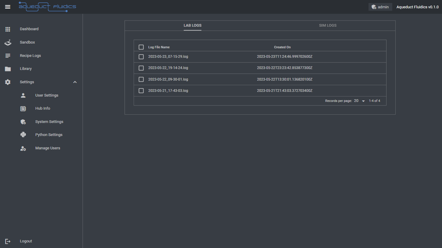
-
On the recipe logs page, you will find two tabs: Sim Logs and Lab Logs. Each tab displays a table with the following columns:
- Log File Name: The name of the recipe log file.
- Created On: The date and time when the log file was created.
-
Viewing Recipe Log Files: To view the contents of a recipe log file, click on the view icon associated with the log file in the table. This will open a viewer that displays the log file's contents, allowing you to inspect the log entries.
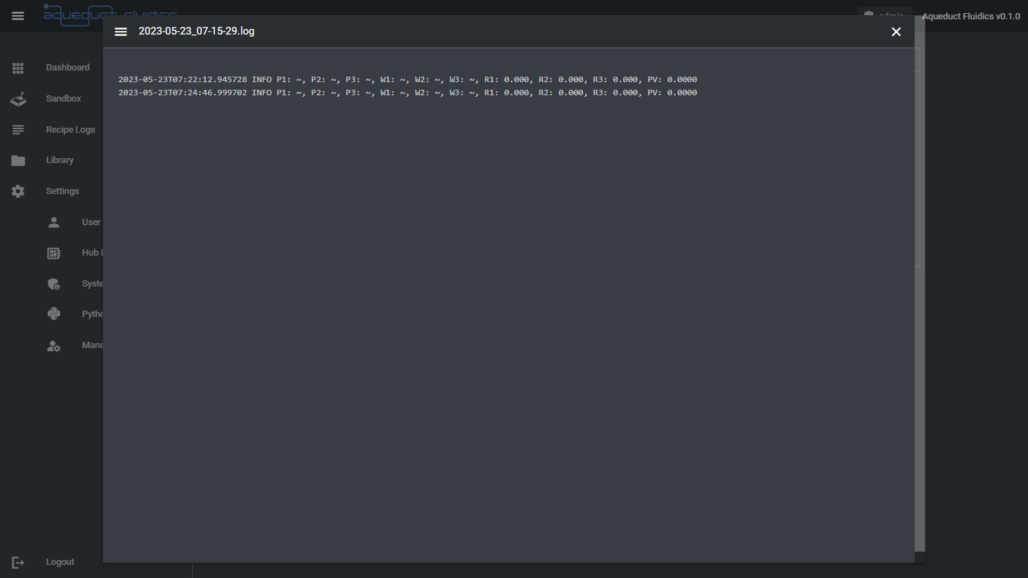
-
Downloading Recipe Log Files: To download a recipe log file, select the row associated with the log file in the table, and then click the download icon at the top right of the table. You can download a single log file with the specified format or multiple log files as a compressed archive (e.g., ZIP).
-
Deleting Recipe Log Files: To delete one or more recipe log files, select the rows associated with the log files in the table, and then click the delete icon at the top right corner of the table. A confirmation prompt will appear to confirm the deletion of the selected log files. Please note that this action permanently removes the log files from the system, so make sure to have backups or copies if you need to retain the log data.

Please note that the availability and accessibility of recipe log files may vary based on your user permissions and the configurations set by the application administrators.
Managing Libraries
The Library page in the Aqueduct dashboard allows you to upload and delete Python libraries for your application.
Navigating to the Library Page
Navigate to the "Library" page by clicking on "Library" in the left-side menu.
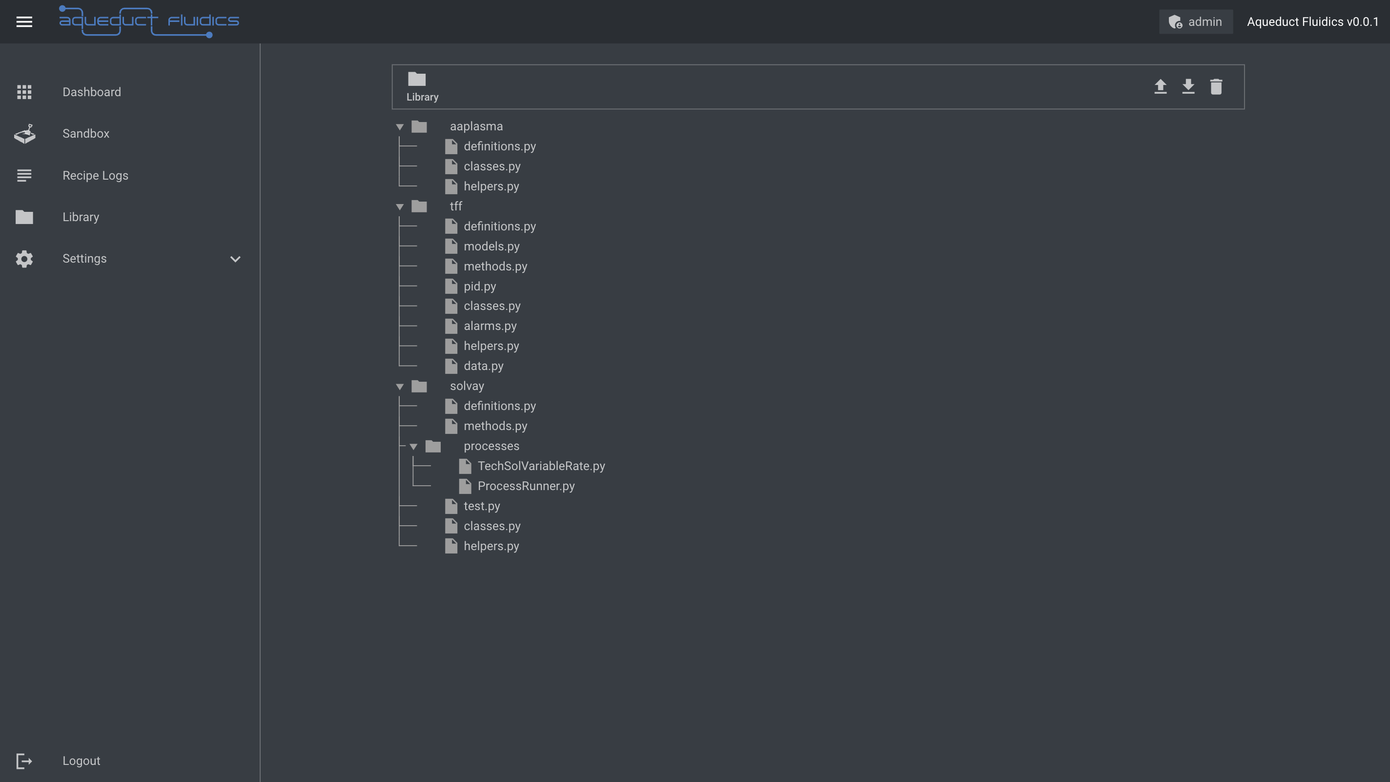
Uploading a Library
To upload a Python library, click on the "Upload" button. A file selection dialog will appear, allowing you to choose the library directory from your local system. Once selected, click "Upload" to initiate the upload process. The library will be added to your library collection and will be available for use in your Aqueduct projects.
Only Python (.py) files will be added.
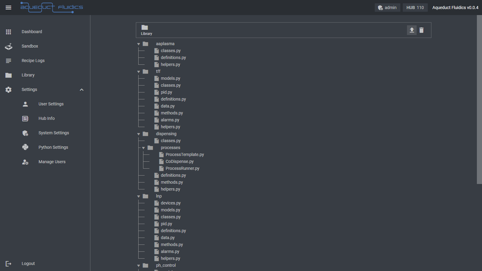
After the upload is complete, a message will display the number of files added with a message like:
successfully uploaded library: wrote 8 files
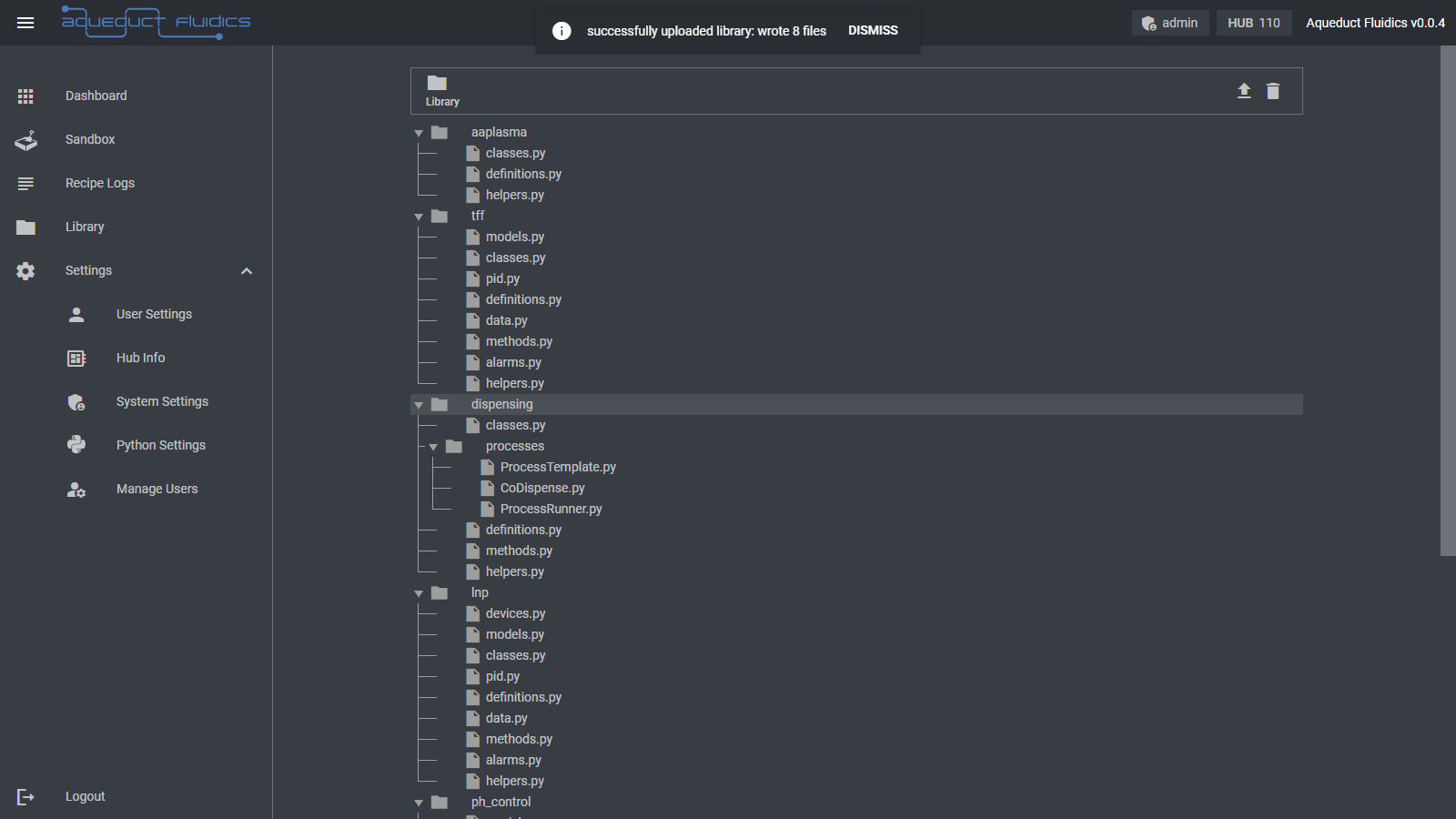
Deleting a Library
To delete a single library, locate the library in the library collection and right click the library name. A context menu will appear. Click the trash can icon to delete the library and then confirm the deletion. Please note that deleting a library will remove it permanently from your library collection, so make sure to backup any important libraries before deletion.
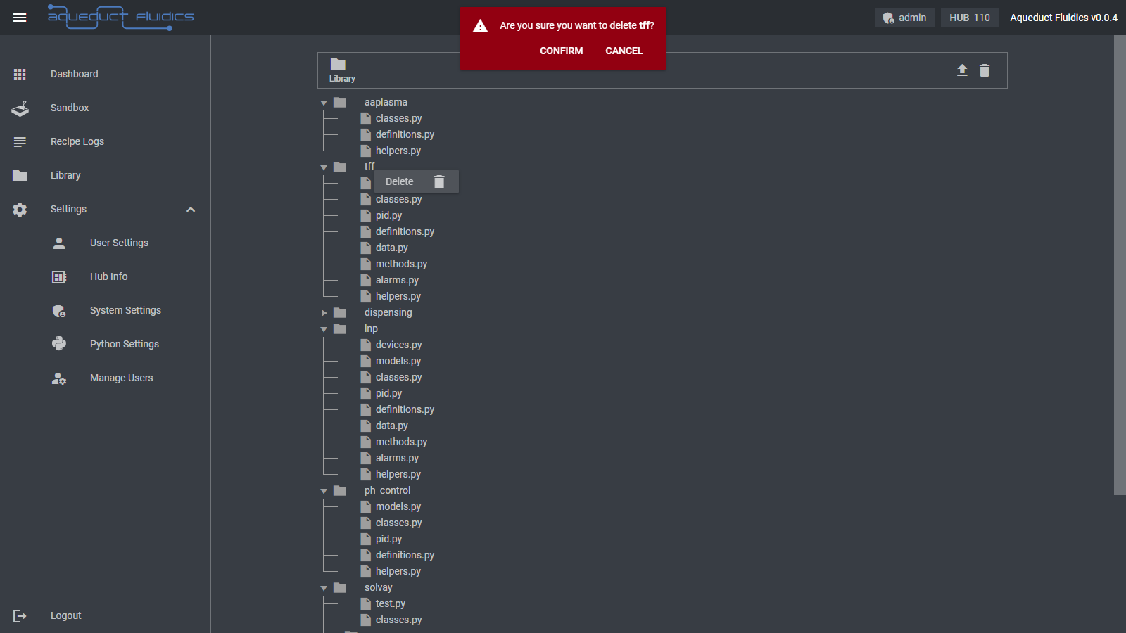
To delete all libraries, click the trash can icon at the top right of the Library file list and then confirm the deletion.
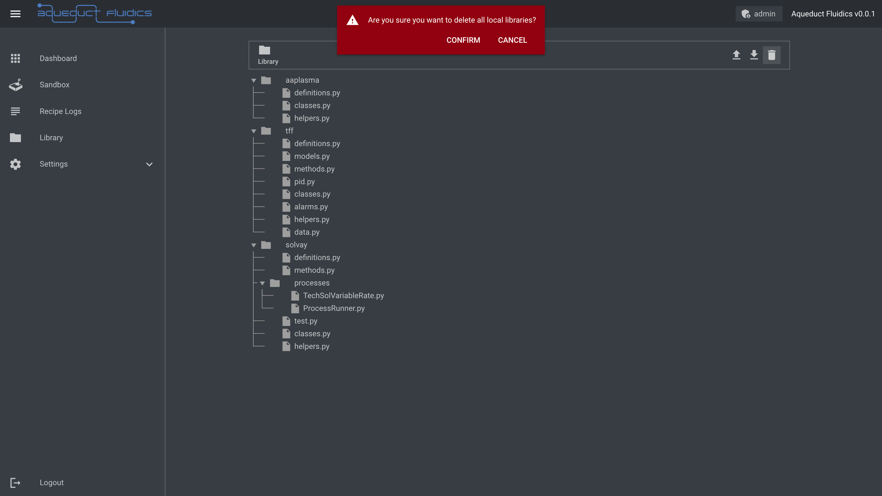
Please note that the availability and accessibility of library management features may vary based on your user permissions and the configurations set by the application administrators.
Managing Settings
The Settings page in the Aqueduct dashboard provides comprehensive control over user and system settings. This page allows you to configure user settings, system settings, view system logs, manage user permissions, and access user logs.
System Settings
System settings provide control over critical aspects of the Aqueduct application. Here, you can perform tasks such as managing application updates, setting the date and time, configuring network interfaces, restarting the application or system, and modifying other system-level parameters. These settings enable you to fine-tune the application to align with your operational needs.
System Logs
The System Logs feature grants access to detailed logs that capture important system events and activities. You can review and analyze these logs to gain insights into the application's behavior, diagnose issues, and track system performance. This helps in troubleshooting, debugging, and ensuring the smooth operation of the Aqueduct application.
User Permissions
The User Permissions functionality allows administrators to manage user access and control permissions within the Aqueduct application. This feature ensures the appropriate level of access and security for different users, granting specific privileges based on their roles and responsibilities. Administrators can assign and revoke permissions, create user groups, and maintain user access control for a secure and streamlined experience.
User Logs
The User Logs section presents a comprehensive log history of user activities within the Aqueduct application. It records events such as login attempts, user settings modifications, system interactions, and other relevant user actions. User logs facilitate auditing, compliance, and accountability, ensuring a transparent and traceable record of user activities.
Please note that the availability and accessibility of settings and features may vary based on your user permissions and the configurations set by the application administrators.
User Settings
In the Aqueduct dashboard, the User Settings section allows you to manage your account information and preferences, including:
- Username: This field displays your username, which is used for login and identification purposes.
- User ID: The User ID is a unique identifier assigned to your user account within the Aqueduct system.
- Role: The Role defines the level of access and permissions assigned to your user account. It determines the actions and features you can access within the application.
- Created at: The Created at timestamp indicates the date and time when your user account was created.
- Password last updated: This field shows the most recent date and time when your account password was updated.
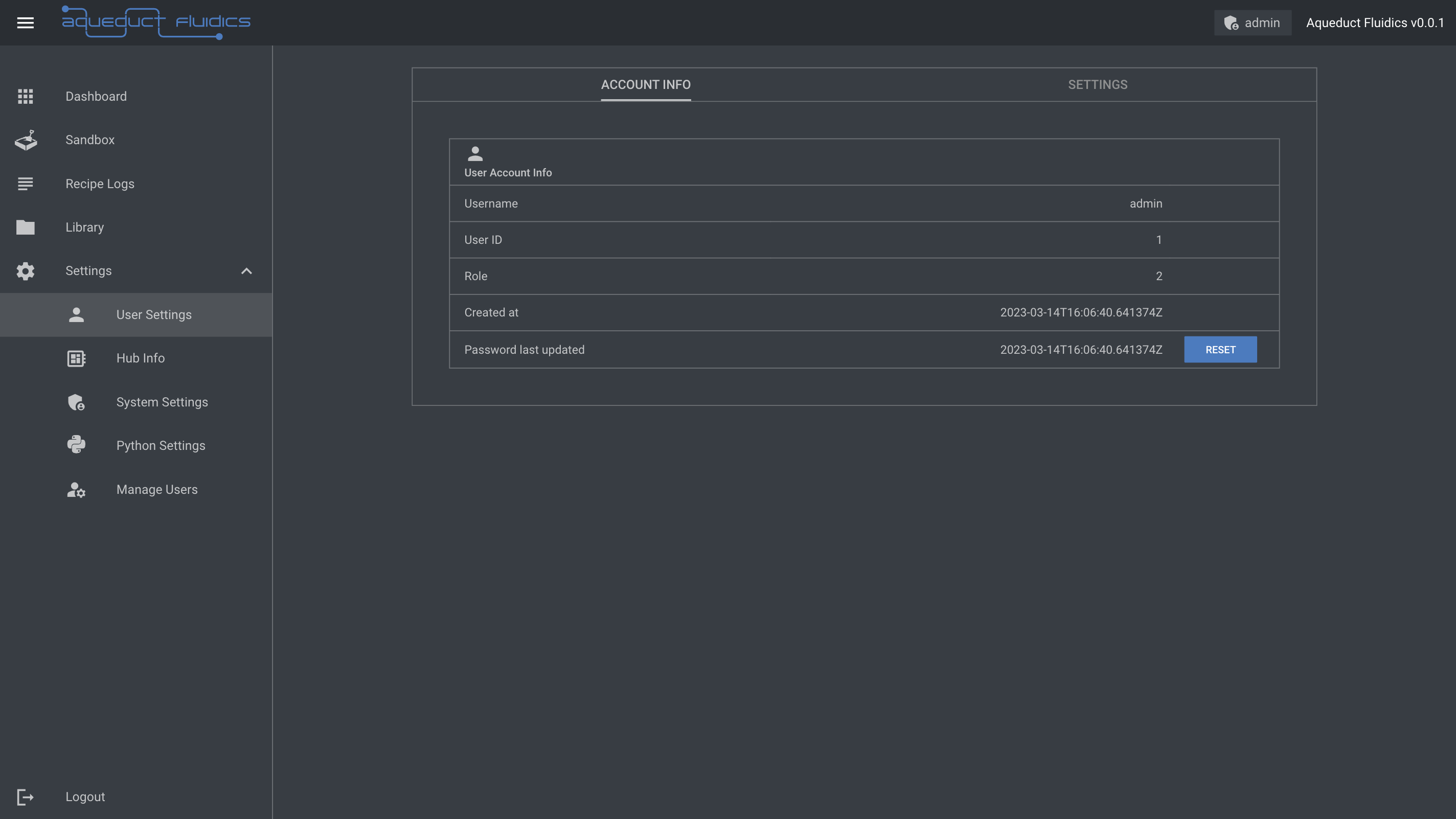
Password Reset
To reset your password, click the "reset" button in the Password last updated row:
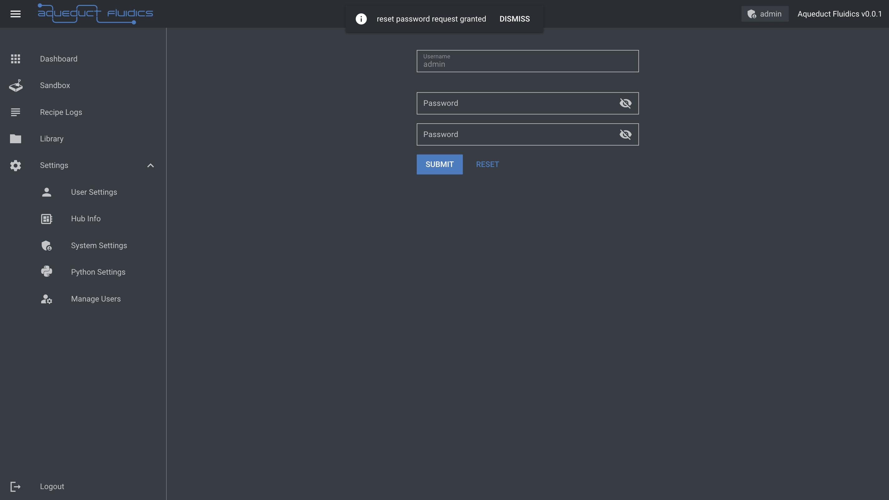
Note: When creating a password, it must:
- Be between 8 and 32 characters long.
- Contain at least one digit.
- Contain at least one uppercase letter.
- Contain at least one lowercase letter.
- Contain at least one symbol.
Managing Hub Info
The Hub Info page in the Aqueduct dashboard provides information about the hub (embedded computer) and allows you to configure certain settings. Here's an overview of the available options:
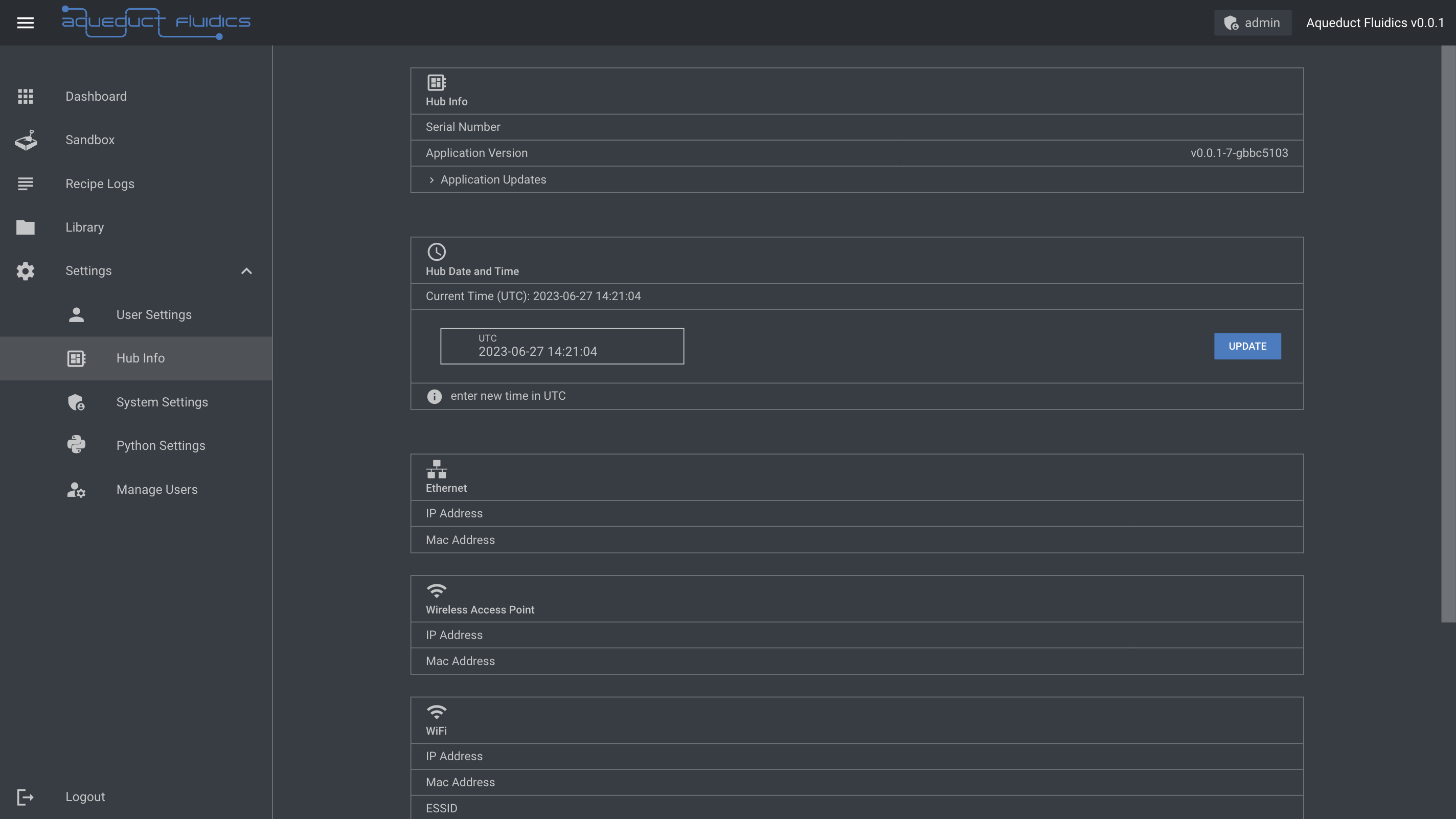
Application Version
- The Application Version section displays the current version of the Aqueduct application running on the hub.
Application Updates
- Clicking on the Application Updates row expands a section where you can upload an update archive for the target system, such as
aqueduct_fluidics-armv7-unknown-linux-musleabihf-0.0.5.zip.
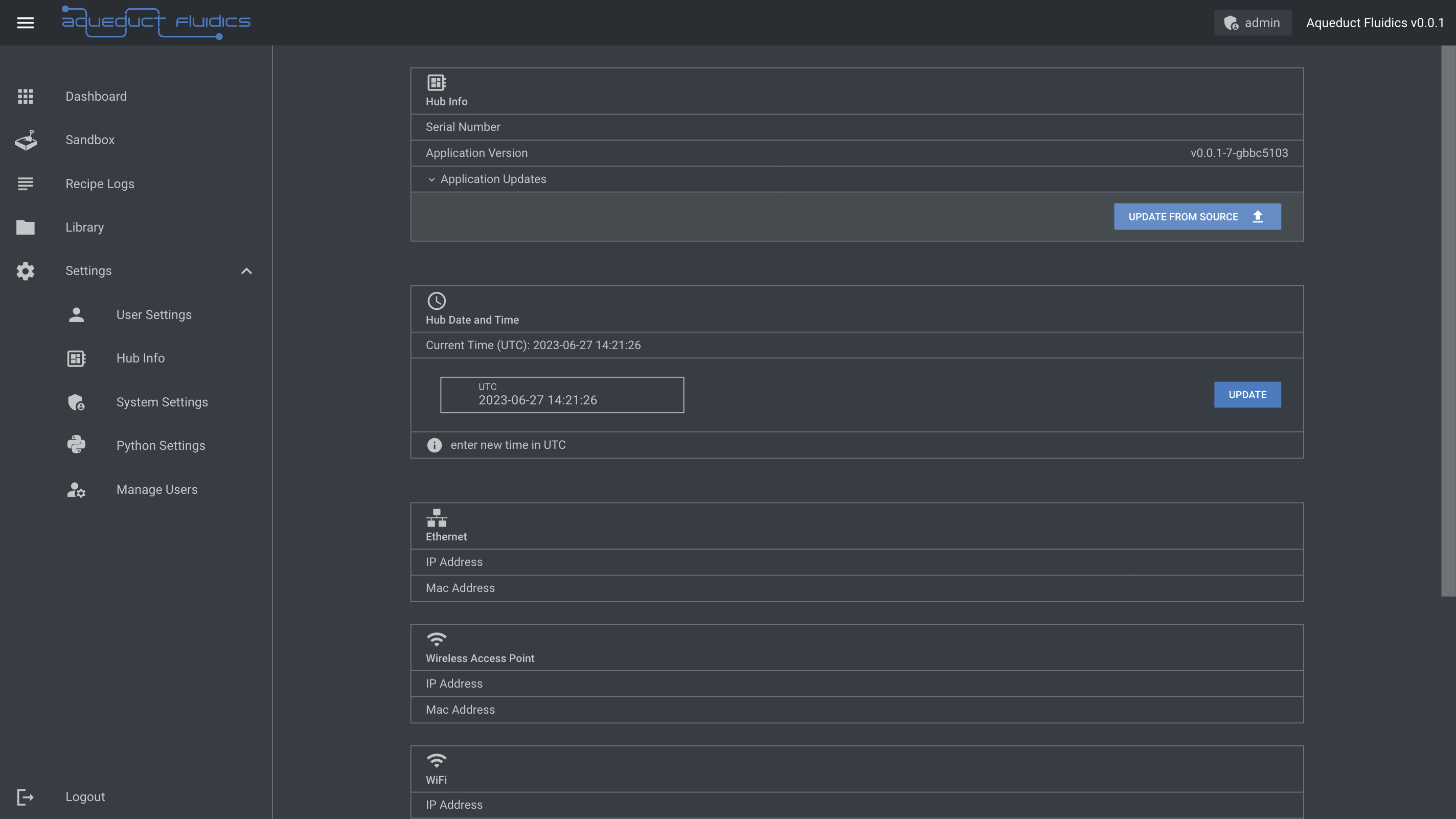
After uploading, you'll see progress updates of the upload and file transfer.
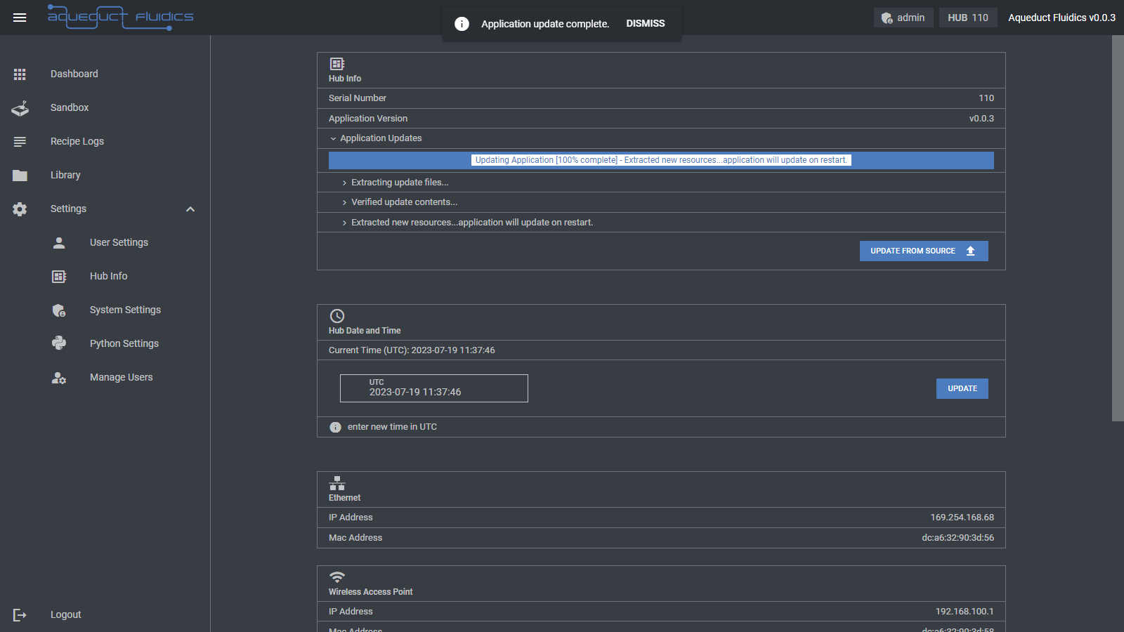
You must restart the application by pressing the Restart Application button for the update to take effect.
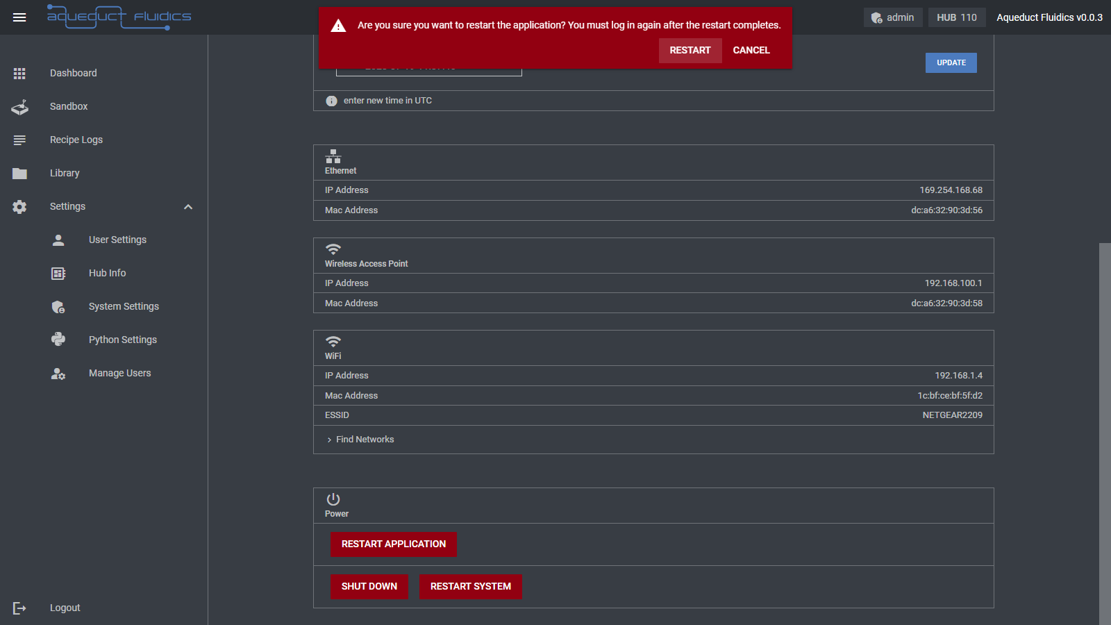
Hub Date and Time
- The Hub Date and Time section allows you to view and update the current date and time settings of the hub.
- Enter a new time value in UTC using the input field provided. Use the
syncbutton to sync the time to the client computer's date and time. - To update the date and time, click the Update button. Please note that this action may require appropriate permissions.
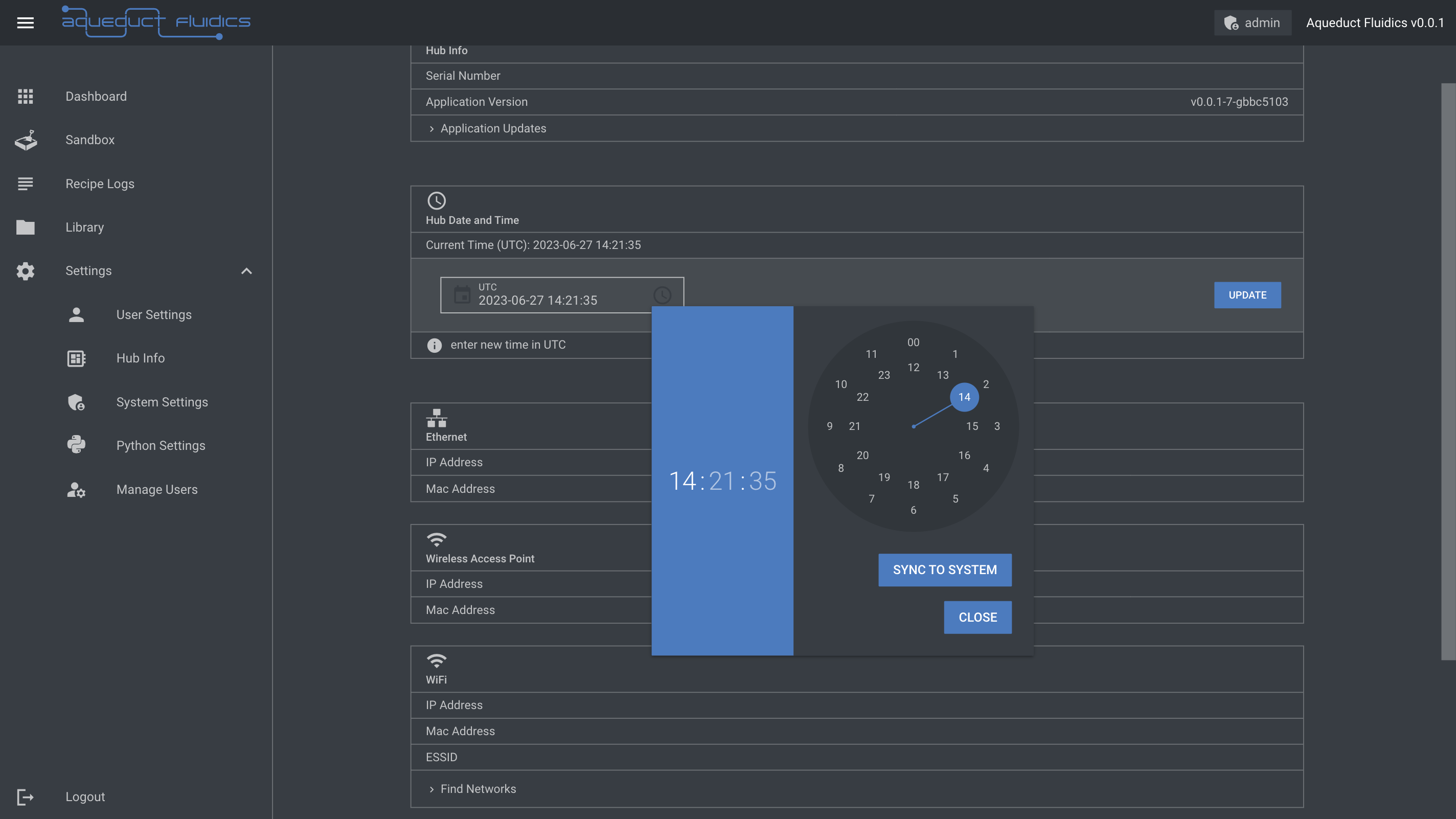
Ethernet
- The Ethernet section displays information related to the hub's Ethernet interface, including the IP address and MAC address.
Wireless Access Point
- The Wireless Access Point section provides information about the hub's wireless access point, including the IP address and MAC address.
- To connect to the hub as a wireless access point, access the network named "HubXXX", where XXX is the hub's serial number.
- The password for the wireless access point is provided to customers.
- The default IP for the hub when accessed as an access point is 192.168.100.1.
WiFi
- The WiFi section displays information about the hub's WiFi connection, including the IP address, MAC address, and ESSID (Extended Service Set Identifier).
- There is also an option to find networks and refresh the WiFi information. This will display available wireless networks that you can connect the hub to.
Power
- The Power section offers options to perform power-related actions on the hub. There are buttons available to:
- restart the application
- shut down the hub (the embedded computer)
- restart the hub (the embedded computer)
System Settings
- Managing Account Creation and Passwords
- Registration Access Code
- Creating a New User Account
- Changing or Resetting a User Password
- Configuring Registration Code Cycling
- Configuring Password Expiration
- Account Lockout
- System Logs
- Logged Events
Managing Account Creation and Passwords
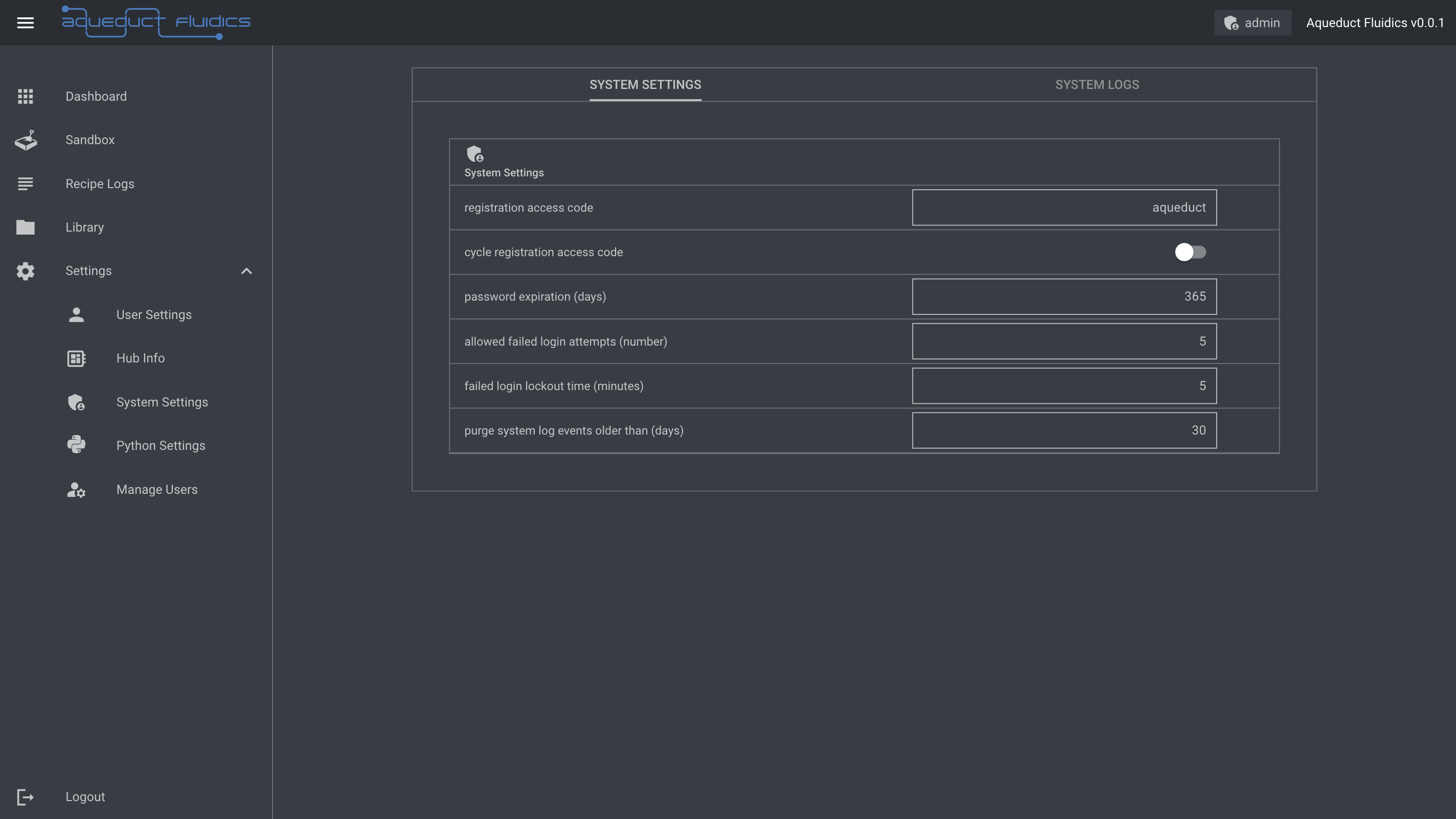
Registration Access Code
- Account creation is restricted by requiring the proper entry of a Registration Access Code.
- The default registration access code is aqueduct, but it can be changed by any user with an admin role in the Hub Settings section of the Dashboard.
- To access the Hub Settings, log in to the admin account and navigate to the Hub Settings link in the Dashboard.
Creating a New User Account
- To create a new user account, go to the sign-in page and click on the Create Account button.
- On the passcode entry screen, enter the Registration Access Code and click Submit.
- After entering the access code, you'll be directed to the account creation screen.
- Enter the desired username and password, then click Create Account to finalize the creation of the new user account.
Note: When creating a password, it must:
- Be between 8 and 32 characters long.
- Contain at least one digit.
- Contain at least one uppercase letter.
- Contain at least one lowercase letter.
- Contain at least one symbol.
Changing or Resetting a User Password
Changing a Password while Logged In
- After logging in, navigate to the My Account section on your Dashboard.
- Click on Reset Password to proceed.
- Enter and confirm a new password in the provided fields at the bottom of the page.
- Click Reset Password to save the new password.
Requesting a Password Reset from an Admin
- If you need to request a password reset, click on the Reset Password link below the Sign-In dialog on the Login page.
- Enter your username in the input field and click Request Password Reset to notify an admin of the request.
Note: An admin must grant permission to reset your password.
- As an admin, navigate to the Users link under the Manage Users heading in the admin Dashboard.
- Select the user who requested a password reset from the table of user accounts.
- Click the Grant button in the row labeled password_update_requested to authorize the password reset.
Configuring Registration Code Cycling
- The application allows for cycling of the Registration Access Code between new user account creation events.
- To configure this feature, go to the Settings link under the Hub Settings section in the admin Dashboard.
- Enter 1 in the Cycle Registration Access Code field to enable code cycling or 0 to disable it.
- Press Update to save the new settings.
Configuring Password Expiration
- The application can enforce password cycling by forcing users to reset their passwords after a specified number of days.
- Configure this duration by navigating to the Settings link under the Hub Settings section in the admin Dashboard.
- Enter the desired password duration (in days) in the Password Expiration (Days) field.
- Press Update to save the new settings.
Account Lockout
- A user account can be locked either by an admin or when the configured number of failed login attempts is exceeded.
Locking a Standard User Account
- To lock a standard user account, go to the Users link under the Manage Users heading in the admin Dashboard.
- Select the user account you want to lock from the table of user accounts.
- Click the Lock button. To unlock the account, repeat the process and click the Unlock button.
Login Failure Lockout
- After a certain number of failed password attempts, a user will be locked out for a specific duration.
- Both the number of allowed failed login attempts and the lockout period can be configured by any user with an admin role.
- Navigate to the Settings link under the Hub Settings section in the admin Dashboard.
- Enter the desired number of allowed failed login attempts and the duration (in minutes) to lock a user account.
- Press Update to save the new settings.
Note: If a user is locked out, an admin can reset the lockout period by going to the Users section under Manage Users in the admin Dashboard. Select the user account that needs a lockout timer reset.
System Logs
The System Logs tab provides access to the logs generated by the Aqueduct system. It offers valuable information about the system's activities, errors, and events, which can be useful for troubleshooting and monitoring purposes.
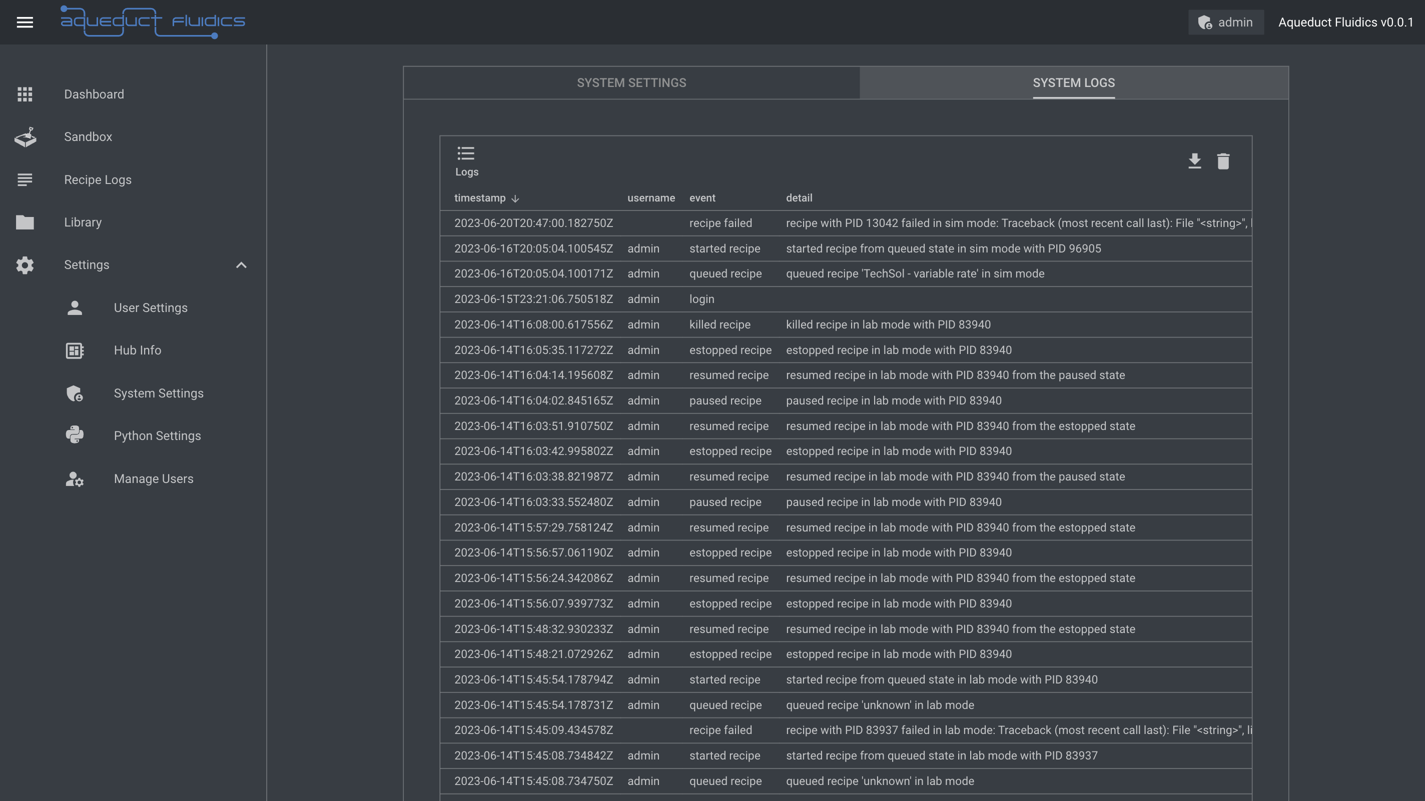
To access the System Logs tab:
- Navigate to the Aqueduct dashboard.
- Click on the System Settings page.
- Click on the System Logs tab.
Within the System Logs tab, you can:
- View a chronological list of system logs.
- Download logs for further analysis or archival purposes.
- Purge logs that are older than the purge system log events older than setting.
Note that access to the System Logs tab may require appropriate permissions or admin-level access to ensure the security and integrity of the system logs.
Logged Events
| Category | Event |
|---|---|
| User Account | Account creation |
| Password change | |
| Password reset requested | |
| Password reset granted | |
| Successful login | |
| Successful logout | |
| Failed login attempt | |
| Account locked or unlocked | |
| Permissions modified | |
| Changed role | |
| System | Changed date and time |
| Shutdown hub | |
| Setups, Recipes, and Libraries | Uploaded local libraries |
| Deleted local libraries | |
| Created setup | |
| Modified setup | |
| Deleted setup | |
| Uploaded setup | |
| Created recipe | |
| Modified recipe | |
| Deleted recipe | |
| Uploaded recipe | |
| Recipe Execution | Queued recipe |
| Started recipe | |
| Resumed recipe | |
| Paused recipe | |
| E-stopped recipe | |
| Recipe failed | |
| Data Access | Downloaded logs |
| Deleted logs |
Python Settings
This page is under construction...
Manage Users
This page is under construction...
Device Types
- Balance
- Mass Flow Meter
- Peristaltic Pump
- pH Probe
- Pinch Valve
- Pressure Transducer
- Solenoid Valve
- Syringe Pump
- Temperature Probe
The Aqueduct Device Types page offers an overview of the different device types supported within the Aqueduct system. Each device type represents a specific category of devices with unique functionalities and capabilities.
Balance

Recorded Data
The Balance records the following attribute during operation:
grams: The weight reading value of the balance in grams.
Python API
The Balance can be controlled and monitored using the Aqueduct Python API. The Python code for interacting with the balance can be found in the aqueduct-py repository.
The balance.py module provides functions and classes to control the balance and retrieve weight readings. You can use this API to perform weight measurements and integrate the balance into your Python applications and automation scripts.
To use the Python API, you can import the Balance class from the balance.py module and create an instance of the balance. Then, you can call the available methods to retrieve weight readings and perform other operations.
Here's an example of how to use the Balance API:
"""Balance Example Script

This script demonstrates the usage of the `Balance` device from the
Aqueduct library. It connects to an Aqueduct instance,
initializes the system, and performs operations on the balance device.
"""
import time

from aqueduct.core.aq import Aqueduct
from aqueduct.core.aq import InitParams
from aqueduct.devices.balance import Balance

# Parse the initialization parameters from the command line
params = InitParams.parse()

# Initialize the Aqueduct instance with the provided parameters
aq = Aqueduct(params.user_id, params.ip_address, params.port)

# Perform system initialization if specified
aq.initialize(params.init)

# Set the command delay for the Aqueduct instance
aq.set_command_delay(0.05)

# Get the balance device from the Aqueduct instance
balance: Balance = aq.devices.get("balance_000001")

# Continuously perform operations on the balance device
while True:
    # Set simulated rates of change for the balance device
    balance_rocs = [5]
    balance.set_sim_rates_of_change(balance_rocs)

    # Get and print the weight readings from the balance device in grams
    print(balance.grams)

    # Pause for 5 seconds
    time.sleep(5)

    # Get and print the weight readings again
    print(balance.grams)

    # Perform a tare operation on the balance device for the first input
    balance.tare(0)
Please refer to the aqueduct-py repository for more details on how to use the Python API with the Balance.
Supported Hardware
- with the Aqueduct 4 x RS232 device node, supports communication with up to 4 Ohaus Adventurer or Scout models via RS232 connectivity (RS232 accessory)
Mass Flow Meter

Recorded Data
The Mass Flow Meter records the following attribute during operation:
ml_min: The mass flow value of the mass flow meter in mL/min.
Python API
The Mass Flow Meter can be controlled and monitored using the Aqueduct Python API. The Python code for interacting with the balance can be found in the aqueduct-py repository.
The meter.py module provides functions and classes to control the mass flow meter and retrieve mass flow readings. You can use this API to perform measurements and integrate the mass flow meter into your Python applications and automation scripts.
To use the Python API, you can import the MassFlowMeter class from the meter.py module and create an instance of the mass flow meter. Then, you can call the available methods to retrieve mass flow readings and perform other operations.
Here's an example of how to use the MassFlowMeter API:
import time

from aqueduct.core.aq import Aqueduct
from aqueduct.core.aq import InitParams
from aqueduct.core.units import MassFlowUnits
from aqueduct.devices.mass_flow import MassFlowMeter

# Parse the initialization parameters from the command line
params = InitParams.parse()

# Initialize the Aqueduct instance with the provided parameters
aq = Aqueduct(params.user_id, params.ip_address, params.port)

# Perform system initialization if specified
aq.initialize(params.init)

# Set the command delay for the Aqueduct instance
aq.set_command_delay(0.05)

# Get the mass flow meter device from the Aqueduct instance
mass_flow_meter: MassFlowMeter = aq.devices.get("mass_flow_meter_000001")

mass_flow_meter.set_sim_values((10.0,), MassFlowUnits.UL_MIN)
mass_flow_meter.set_sim_rates_of_change((0.5,), MassFlowUnits.UL_MIN)

# Continuously perform operations on the mass flow meter devices
while True:
    # Get and print the mass flow reading from the mass flow meter device
    print(f"Mass Flow: {mass_flow_meter.ul_min[0]:.3f}ul/min")

    # Pause for 5 seconds
    time.sleep(5)
Please refer to the aqueduct-py repository for more details on how to use the Python API with the Mass Flow Meter.
Supported Hardware
Peristaltic Pump

Recorded Data
The Peristaltic Pump records the following attributes during operation:
ml_target: The target volume in milliliters (ml) for the pump operation.ml_done: The volume in milliliters (ml) that has been pumped so far.ml_min: The current pump rate in milliliters per minute (ml/min).status: The status of the peristaltic pump. It is represented as a u8 value and can have one of the following values:0: Stopped1: Clockwise2: CounterClockwise
mode: The operational mode of the peristaltic pump. It is represented as a u8 value and can have one of the following values:0: Continuous1: Finite
Python API
The Peristaltic Pump can be controlled using the Aqueduct Python API. The Python code for interacting with the peristaltic pump can be found in the aqueduct-py repository.
The peristaltic.py module provides functions and classes to control the peristaltic pump. You can use this API to set the target volume, monitor the pump status, and control the operational mode. The API allows you to integrate the peristaltic pump into your Python applications and automation scripts.
To use the Python API, you can import the PeristalticPump class from the peristaltic.py module and create an instance of the pump. Then, you can call the available methods to control and monitor the pump's operation.
"""A module for controlling peristaltic pumps using the Aqueduct framework.

This demo program initializes a PeristalticPump device, sets the pump to run
continuously at a specific flow rate, and then reverses the direction of the
pump's rotation after a certain amount of time has passed. The program continuously
checks the flow rate of the pump and sends new start commands to reverse
the direction if the flow rate reaches 0.
"""
from aqueduct.core.aq import Aqueduct
from aqueduct.core.aq import InitParams
from aqueduct.devices.pump import PeristalticPump

# parse initialization parameters and create Aqueduct instance
params = InitParams.parse()
aq = Aqueduct(params.user_id, params.ip_address, params.port)

# initialize the devices and set a command delay
aq.initialize(params.init)
aq.set_command_delay(0.05)

# get the peristaltic pump device and create a command object
pump: PeristalticPump = aq.devices.get("peristaltic_pump_000001")
commands = pump.make_commands()
c = pump.make_start_command(
    mode=pump.MODE.Continuous,
    rate_units=pump.RATE_UNITS.MlMin,
    rate_value=2,
    direction=pump.STATUS.Clockwise,
)

# set the command for each channel and start the pump
for i in range(0, pump.len):
    pump.set_command(commands, i, c)

pump.start(commands)

# set the maximum speed and speed increment for the pump
MAX_SPEED: float = 50
INCREMENT: float = 0.1

# calculate the number of steps based on the maximum speed and increment
STEPS = int(MAX_SPEED / INCREMENT)

# loop through the speed increment steps
while True:
    for i in range(0, STEPS):
        commands = pump.make_commands()

        # create a command to change the pump speed
        c = pump.make_change_speed_command(
            rate_value=i * INCREMENT, rate_units=pump.RATE_UNITS.MlMin
        )

        # set the command for each channel and change the pump speed
        for i in range(0, pump.len):
            pump.set_command(commands, i, c)

        pump.change_speed(commands)

    # loop through the speed decrement steps
    for i in range(STEPS, 0, -1):
        commands = pump.make_commands()

        # create a command to change the pump speed
        c = pump.make_change_speed_command(
            rate_value=i * INCREMENT, rate_units=pump.RATE_UNITS.MlMin
        )

        # set the command for each channel and change the pump speed
        for i in range(0, pump.len):
            pump.set_command(commands, i, c)

        pump.change_speed(commands)
Please refer to the aqueduct-py repository for more details on how to use the Python API with the Peristaltic Pump.
E-Stop Behavior
In the Aqueduct system, pressing the E-Stop button has a specific behavior for peristaltic pumps:
- When the Aqueduct E-Stop button is pressed, all peristaltic pumps will immediately stop their operation.
- Upon resumption, the operator will have the option to manually resume the pump's operation by selecting the appropriate control settings.
Supported Hardware
-
with the Masterflex L/S® Mixed Signal (4-20mA I/O, isolated DIO) device node, supports control of a single Masterflex L/S® Pump
-
with the Stepper Motor device node, supports control of a single Boxer 9QQ/15QQ Pump
-
with the 2x Can + 2x RS485 device node, supports control of six Boxer 9QQ/15QQ Pumps via Can or RS485
pH Probe

Recorded Data
ph: : The pH value of the probe input.
Python API
"""pH Probe Example Script

This script demonstrates the usage of the `PhProbe` device from the
Aqueduct library. It connects to an Aqueduct instance,
initializes the system, and performs operations on the pH probe device.
"""
import time

from aqueduct.core.aq import Aqueduct
from aqueduct.core.aq import InitParams
from aqueduct.devices.ph import PhProbe

# Parse the initialization parameters from the command line
params = InitParams.parse()

# Initialize the Aqueduct instance with the provided parameters
aq = Aqueduct(params.user_id, params.ip_address, params.port)

# Perform system initialization if specified
aq.initialize(params.init)

# Set the command delay for the Aqueduct instance
aq.set_command_delay(0.05)

# Get the pH probe device from the Aqueduct instance
ph_probe: PhProbe = aq.devices.get("ph_probe_000001")

# Continuously perform operations on the pH probe device
while True:
    # Get and print the pH reading from the pH probe device
    ph_value = ph_probe.ph
    print(f"pH: {ph_value}")

    # Pause for 5 seconds
    time.sleep(5)
Please refer to the aqueduct-py repository for more details on how to use the Python API with the pH Probe.
Supported Hardware
- with the Aqueduct 3x pH Probe A/D device node, supports reading and calibration of 3 pH eletrodes
Pinch Valve

Recorded Data
The Pinch Valve records the following attribute during operation:
pct_open: The position of the pinch valve. It is represented as a floating-point value ranging from 0.0 to 1.0. A value of 1.0 represents the valve being completely open.
Python API
"""PinchValve demo.

This demo program initializes a PinchValve device, sets it to gradually open and close
over a range of values from 0 to 100 and back down to 0. The program continuously
checks the position of the valve and sends new position commands to gradually change
the valve's position. The time delay between position changes is decreased from
0.1 seconds to 0.001 seconds in increments of 10x to create a more gradual transition.
During each loop, the current position of the valve is printed to the console.
"""
import time

from aqueduct.core.aq import Aqueduct
from aqueduct.core.aq import InitParams
from aqueduct.devices.valve.pinch import PinchValve

params = InitParams.parse()
aq = Aqueduct(params.user_id, params.ip_address, params.port)
aq.initialize(params.init)

# get the PinchValve device
pinch_valve: PinchValve = aq.devices.get("pinch_valve_000001")

# continuously cycle through opening and closing the valve
while True:

    # loop through various sleep times to change the speed of valve movement
    for sleep in (0.001, 0.01, 0.1):

        # loop through the valve position values from 0 to 100 percent open
        for i in range(0, 100):
            commands = pinch_valve.make_commands()
            c = pinch_valve.make_set_position_command(pct_open=i / 100.0)
            pinch_valve.set_command(commands, 0, c)
            pinch_valve.set_position(commands, record=True)
            print(pinch_valve.get_pct_open())
            time.sleep(sleep)

        # loop through the valve position values from 100 to 0 percent open
        for i in range(100, 0, -1):
            commands = pinch_valve.make_commands()
            c = pinch_valve.make_set_position_command(pct_open=i / 100.0)
            pinch_valve.set_command(commands, 0, c)
            pinch_valve.set_position(commands, record=True)
            print(pinch_valve.get_pct_open())
            time.sleep(sleep)
Please refer to the aqueduct-py repository for more details on how to use the Python API with the Pinch Valve.
Supported Hardware
- with the Aqueduct Motor Driver device node, supports control of a stepper motor driven pinch valve
Pressure Transducer

Recorded Data
The Pressure Transducer captures the following recorded data during operation:
torr: The pressure reading from the transducer in units oftorr. This field provides real-time pressure information.
Python API
The Pressure Transducer can be controlled and accessed using the Python API provided by the manufacturer. The Python code for interacting with the Pressure Transducer can be found in the aqueduct-py repository.
"""Pressure Transducer Example Script

This script demonstrates the usage of the `PressureTransducer` device from the
Aqueduct library. It connects to an Aqueduct instance,
initializes the system, and performs operations on the pressure transducer device.
"""
import time

from aqueduct.core.aq import Aqueduct
from aqueduct.core.aq import InitParams
from aqueduct.core.units import PressureUnits
from aqueduct.devices.pressure import PressureTransducer

# Parse the initialization parameters from the command line
params = InitParams.parse()

# Initialize the Aqueduct instance with the provided parameters
aq = Aqueduct(params.user_id, params.ip_address, params.port)

# Perform system initialization if specified
aq.initialize(params.init)

# Set the command delay for the Aqueduct instance
aq.set_command_delay(0.05)

# Get the pressure transducer device from the Aqueduct instance
pressure_transducer: PressureTransducer = aq.devices.get("pressure_transducer_000001")

pressure_transducer.set_sim_roc((1,), units=PressureUnits.PSI)

# Continuously perform operations on the pressure transducer device
while True:
    # Get and print the pressure reading from the pressure transducer device
    pressure_value = pressure_transducer.torr
    print(f"Pressure: {pressure_value}")

    # Pause for 5 seconds
    time.sleep(5)
Supported Hardware
- with the Aqueduct 4 x RS232 device node, supports communication with up to 12 Parker SciLog SciPres transducers via RS232 connectivity
Solenoid Valve

Recorded Data
Python API
"""SolenoidValve demo.

This demo program initializes a SolenoidValve device and repeatedly toggles the position.
"""
import time

from aqueduct.core.aq import Aqueduct
from aqueduct.core.aq import InitParams
from aqueduct.devices.valve.solenoid import SolenoidValve

params = InitParams.parse()
aq = Aqueduct(params.user_id, params.ip_address, params.port)
aq.initialize(params.init)

# get the SolenoidValve device
solenoid_valve: SolenoidValve = aq.devices.get("solenoid_valve_000001")

# continuously cycle through toggling the valve
while True:

    commands = solenoid_valve.make_commands()
    c = solenoid_valve.make_set_position_command(position=0)
    solenoid_valve.set_command(commands, 0, c)
    solenoid_valve.set_position(commands, record=True)
    print(solenoid_valve.get_position())

    time.sleep(2)

    commands = solenoid_valve.make_commands()
    c = solenoid_valve.make_set_position_command(position=1)
    solenoid_valve.set_command(commands, 0, c)
    solenoid_valve.set_position(commands, record=True)
    print(solenoid_valve.get_position())

    time.sleep(2)
Please refer to the aqueduct-py repository for more details on how to use the Python API with the Solenoid Valve.
Supported Hardware
- with the Aqueduct 12 x 24V Solenoid Driver device node, supports control of up to 12 solenoids
Syringe Pump

Recorded Data
The Syringe Pump records the following attributes during operation:
status: The status of the syringe pump. It is represented as a u8 value and can have one of the following values:0: Stopped1: Infusing2: Withdrawing3: Paused
mode: The operational mode of the syringe pump. It is represented as a u8 value and can have one of the following values:0: Continuous1: Finite
ul_min: The current infusion or withdrawal rate of the pump in microliters per minute (uL/min). The value is always positive.finite_value: The target volume to dispense or withdraw when operating in Finite mode. The value is always positive.finite_units: The units of the target volume to dispense or withdraw when operating in Finite mode. It is represented as a u8 value.finite_ul_target: The target volume in microliters (uL) to dispense or withdraw when operating in Finite mode.finite_ul_infused: The volume in microliters (uL) infused so far when operating in Finite mode.finite_ul_withdrawn: The volume in microliters (uL) withdrawn so far when operating in Finite mode.position: The plunger position of the syringe pump, ranging from 0 to 1. A value of 0 indicates the fully infused position, and a value of 1 indicates the fully withdrawn position.position_target: The plunger target position of the syringe pump, ranging from 0 to 1. A value of 0 indicates the fully infused position, and a value of 1 indicates the fully withdrawn position.valve_position: The valve position of the syringe pump. The mapping of the position to a port depends on the valve configuration.plunger_mode: The plunger positioning mode of the syringe pump. Not all configurations utilize this field. It is represented as a u8 value.
Python API
The Syringe Pump can be controlled using the Aqueduct Python API. The Python code for interacting with the syringe pump can be found in the aqueduct-py repository.
The syringe.py module provides functions and classes to control the syringe pump. You can use this API to set the infusion rate, target volume, and operational mode. The API allows you to integrate the syringe pump into your Python applications and automation scripts.
To use the Python API, you can import the SyringePump class from the syringe.py module and create an instance of the pump. Then, you can call the available methods to control and monitor the pump's operation.
"""SyringePump demo.

This demo program initializes a SyringePump device, sets
the pump to run continuously at increasing flow rates,
and then reverses the direction of each pump input one by
one as it reaches 0 flow rate. The program continuously
checks the flow rates of each pump input and sends new start
commands to reverse the direction if the flow rate
reaches 0.
"""
# import necessary modules
import time
from typing import List

from aqueduct.core.aq import Aqueduct
from aqueduct.core.aq import InitParams
from aqueduct.devices.pump.syringe import Status
from aqueduct.devices.pump.syringe import SyringePump

# get initialization parameters
params = InitParams.parse()
# create an instance of the Aqueduct API with the given user_id, ip_address and port
aq = Aqueduct(params.user_id, params.ip_address, params.port)
# initialize the pump
aq.initialize(params.init)
# set a delay between sending commands to the pump
aq.set_command_delay(0.05)

# get the SyringePump device
pump: SyringePump = aq.devices.get("syringe_pump_000001")
# create a list to store the last direction used for each pump
last_directions: List[Status] = []

commands = pump.make_commands()
# create start commands for each pump at increasing rates
for i in range(0, pump.len):
    # create a command to set the pump to continuous mode, with a rate of i+1 ml/min, infusing
    c = pump.make_start_command(
        mode=pump.MODE.Finite,
        rate_units=pump.RATE_UNITS.MlMin,
        rate_value=i + 1,
        direction=pump.STATUS.Infusing,
        finite_units=pump.FINITE_UNITS.Ml,
        finite_value=1.0,
    )
    # store the direction used for this command
    last_directions.append(pump.STATUS.Infusing)
    # set the command for this pump
    pump.set_command(commands, i, c)

# start the pumps
pump.start(commands)

while True:
    # get the flow rates for each pump
    ul_min = pump.get_ul_min()
    # create a new list of commands for each pump
    commands = pump.make_commands()
    # check if any pumps have a flow rate of 0, and if so, reverse their direction
    for i, s in enumerate(ul_min):
        if ul_min[i] == 0:
            # reverse the direction of this pump
            d = last_directions[i].reverse()
            # create a new command with the reversed direction
            c = pump.make_start_command(
                mode=pump.MODE.Continuous,
                rate_units=pump.RATE_UNITS.MlMin,
                rate_value=i + 1,
                direction=d,
                finite_units=pump.FINITE_UNITS.Ml,
                finite_value=1.0,
            )
            # update the last direction used for this pump
            last_directions[i] = d
            # set the new command for this pump
            pump.set_command(commands, i, c)
    # start the pumps with the new commands
    pump.start(commands)
    # wait for a short time before checking again
    time.sleep(0.05)
Please refer to the aqueduct-py repository for more details on how to use the Python API with the Syringe Pump.
E-Stop Behavior
In the Aqueduct system, pressing the E-Stop button has a specific behavior for syringe pumps:
- When the Aqueduct E-Stop button is pressed, all syringe pumps will immediately stop their operation.
- Upon resumption, the operator will have the option to manually resume the pump's operation by selecting the appropriate control settings.
Supported Hardware
- with the 2x Can + 2x RS485 device node, supports control of up to 16 TriContinent C(X) series syringe pumps
Temperature Probe

Recorded Data
The Temperature Probe records the following attribute during operation:
celcius: The temperature value measured by the temperature probe in degrees Celsius.
Python API
The Temperature Probe can be controlled and monitored using the Aqueduct Python API. The Python code for interacting with the temperature probe can be found in the aqueduct-py repository.
The probe.py module provides functions and classes to control the temperature probe and retrieve temperature readings. You can use this API to perform temperature measurements and integrate the temperature probe into your Python applications and automation scripts.
To use the Python API, you can import the TemperatureProbe class from the probe.py module and create an instance of the temperature probe. Then, you can call the available methods to retrieve temperature readings and perform other operations.
Here's an example of how to use the TemperatureProbe API:
import time

from aqueduct.core.aq import Aqueduct
from aqueduct.core.aq import InitParams
from aqueduct.core.units import TemperatureUnits
from aqueduct.devices.temperature import TemperatureProbe

# Parse the initialization parameters from the command line
params = InitParams.parse()

# Initialize the Aqueduct instance with the provided parameters
aq = Aqueduct(params.user_id, params.ip_address, params.port)

# Perform system initialization if specified
aq.initialize(params.init)

# Set the command delay for the Aqueduct instance
aq.set_command_delay(0.05)

# Get the temperature probe device from the Aqueduct instance
temperature_probe: TemperatureProbe = aq.devices.get("temperature_probe_000001")

temperature_probe.set_sim_values((25.0,), TemperatureUnits.FAHRENHEIT)

temperature_probe.set_sim_rates_of_change((1.0,), TemperatureUnits.FAHRENHEIT)

# Continuously perform operations on the temperature probe device
while True:
    # Get and print the temperature reading from the temperature probe device
    print(
        f"Temperature: {temperature_probe.fahrenheit[0]:.3f}F, "
        f"{temperature_probe.celsius[0]:.3f}C"
    )

    # Pause for 5 seconds
    time.sleep(5)
Please refer to the aqueduct-py repository for more details on how to use the Python API with the Temperature Probe.
Supported Hardware
Overview
Balances
Mass Flow Meters
Peristaltic Pumps
Pinch Valves
pH Probes
Pressure Transducers
Syringe Pumps
Balances
Ohaus Adventurer & Scout
Table of Contents
- Device Specifications
- Connection and Setup
- Ohaus Adventurer® Configuration
- Integration with Aqueduct System
Device Specifications
| Feature | Value |
|---|---|
| Balance Type | Adventurer® PRECISION AX8201/E |
| Maximum Capacity | 8,200 g |
| Readability | 0.1 g |
| Pan Size | 7.7 in x 6.9 in (195 mm x 175 mm) |
| Minimum Weight (USP, 0.1%, typical) | 200 g |
| Repeatability (typical) | 0.1 g |
| Stabilization Time | 1.5 s |
For complete specs, see Ohaus's documentation here.
Connection and Setup
Connect up to four Ohaus Adventurer® balances to the Aqueduct Ohaus Adventurer Device Node with a straight-through, male-to-male DB-9 cable. Then, connect the Device Node to an Aqueduct Hub using an Aqueduct CommCable.
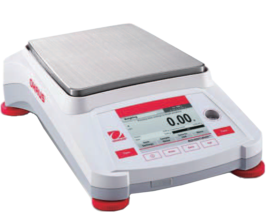
|
Ohaus Adventurer® Configuration
To properly interface with the Device Node, several configuration settings must be changed on the Ohaus Adventurer® balance.
Main Menu
Use the touchscreen display to navigate to the Main Menu.
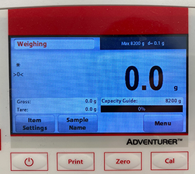
|
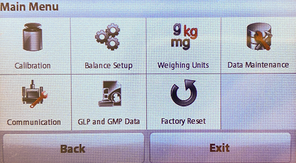
|
Communication Settings
Set the following communication settings on the Ohaus Adventurer® balance:
-
Set the RS232 protocol to 8NI:
- Main Menu > Communication > RS232 Standard > Transmission > 8NI
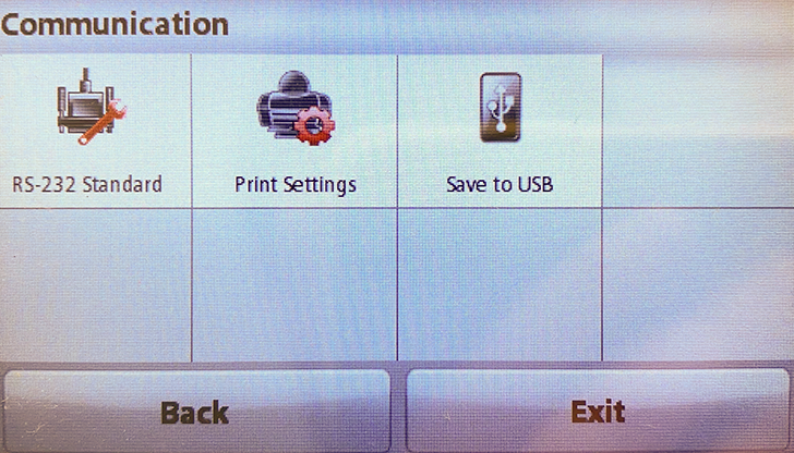
|
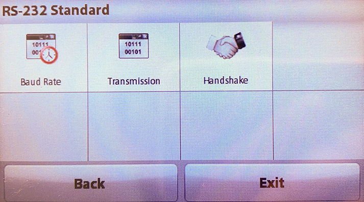
|
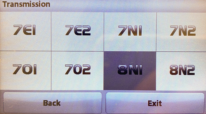
|
-
Set the RS232 handshake to None:
- Main Menu > Communication > RS232 Standard > Handshake > None
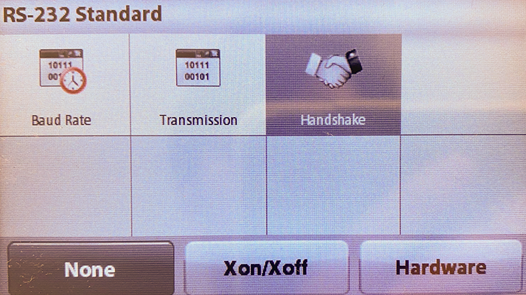
|
-
Set the Print Output to Numeric Value Only:
- Main Menu > Communication > Print Settings > Print Output > Numeric Value Only > ON
|
|
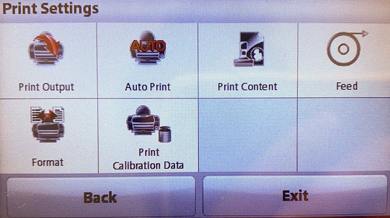
|
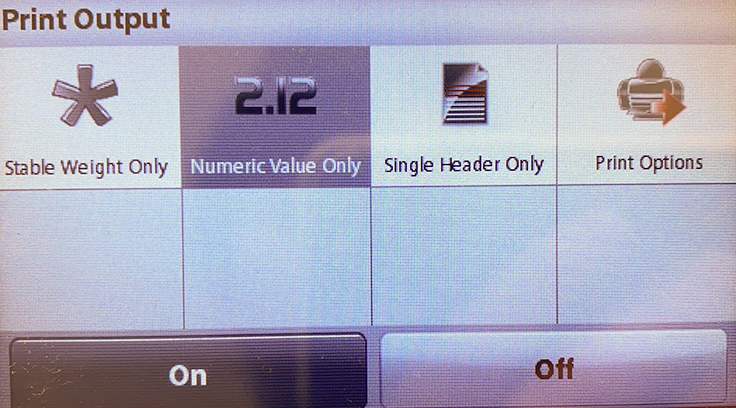
|
-
Set the Print Output to PC:
- Main Menu > Communication > Print Settings > Print Output > Print Options > PC
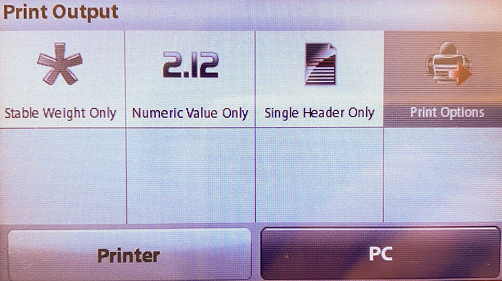
|
-
Set the Auto Print Interval to 1 second:
- Main Menu > Communication > Print Settings > Auto Print > Interval > 1 second
|
|
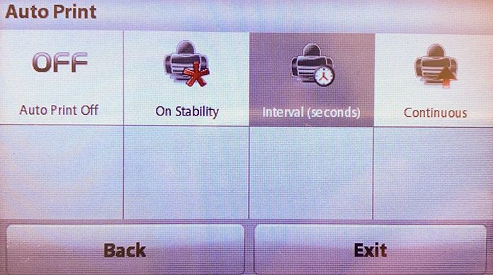
|
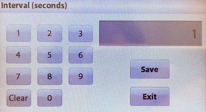
|
-
Set the Print Settings Feed to 1 Line:
- Main Menu > Communication > Print Settings > Feed > 1 Line
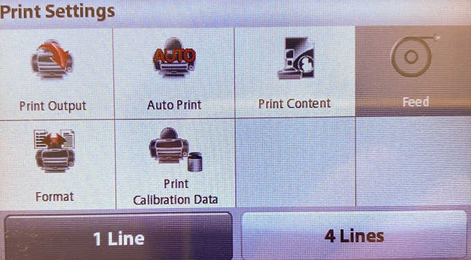
|
- Set the Print Settings Format to Single Line:
- Main Menu > Communication > Print Settings > Format > Single Line
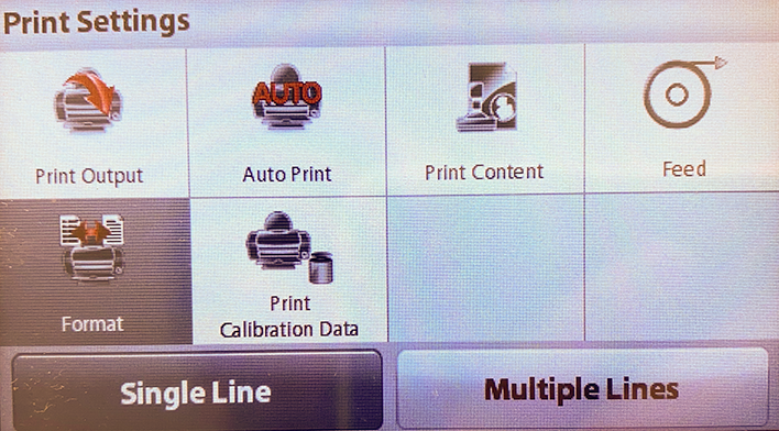
|
Integration with Aqueduct System
Integrate your Ohaus Adventurer® balances into the Aqueduct system with the Aqueduct Fluidics Ohaus Adventurer® Device Node.
The Aqueduct Device Node enables monitoring or recording of the mass measured by up to four (4) balances. The values can be used in Recipe scripts.
Mass Flow Meters
Bronkhorst Coriflow
This page is under construction...
Peristaltic Pumps
Masterflex L/S® Peristaltic Pump
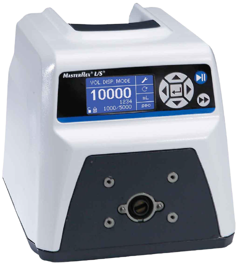
The Masterflex L/S® peristaltic pump is a versatile and reliable pump designed for fluid handling applications. It offers precise control over flow rates and is commonly used in laboratory and industrial settings. This readme provides important information and instructions for setting up and operating the Masterflex L/S® pump with the Aqueduct system.
Specifications
| Feature | Value |
|---|---|
| Pump Series | L/S |
| Control Type | Digital Variable Speed |
| Min RPM (rpm) | 0.1 |
| Max RPM (rpm) | 600 |
| Speed | Variable |
| Speed Control | ±0.1% (0.1 rpm at 600 rpm) |
| Max Flow Rate (mL/min) | 3400 |
| Min Flow Rate (mL/min) | 0.006 |
| Directionality | Bi-directional (Reversible motor) |
For complete specifications, see Cole-Parmer's documentation here.
Setup and Connection
To connect the Masterflex L/S® peristaltic pump to the Aqueduct system, follow these steps:
- Connect the Cole-Parmer Masterflex L/S® peristaltic pump to the Aqueduct Masterflex L/S® Mixed Signal (4-20mA I/O, isolated DIO) Node using a straight-through, shielded DB-25 cable.
- Connect the Masterflex Device Node to an Aqueduct Hub using an Aqueduct CommCable.
Configuration
To properly interface with the Device Node, several configuration settings must be changed on the Masterflex L/S® peristaltic pump. Follow these steps:
Remote Start/Stop
- With the Masterflex L/S® pump powered on, press the Enter button to view the Settings Menu.
- Use the Up and Down arrows to select START/STOP. Press Enter.
- Select ON. Press Enter.
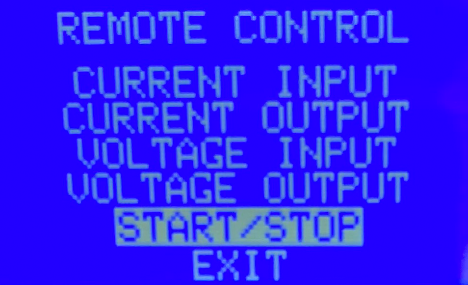
|
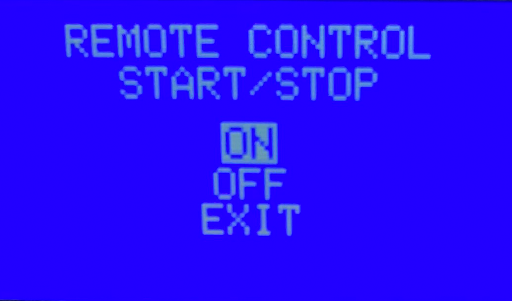
|
Update Current Input
- Return to the main Settings Menu. Use the Up and Down arrows to select CURRENT INPUT. Press Enter.
- Use the Up and Down arrows to set MIN. 4.2 mA = 0.0 mL/min. Press Enter.
- Use the Up and Down arrows to navigate to MAX.
- Assign your desired maximum flow rate to 19.7 mA. For instance, if you wish to achieve a maximum flow rate of 100 mL/min, set MAX. 19.7 mA = 100.0 mL/min. Press Enter.
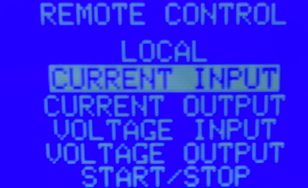
|
Update Current Output
- Return to the main Settings Menu. Use the Up and Down arrows to select CURRENT OUTPUT. Press Enter.
- Use the Up and Down arrows to set MIN. 4.2 mA = 0.0 mL/min. Press Enter.
- Use the Up and Down arrows to navigate to MAX.
- Assign your desired maximum flow rate to 19.7 mA. For instance, if you wish to achieve a maximum flow rate of 100 mL/min, set MAX. 19.7 mA = 100.0 mL/min. Press Enter.
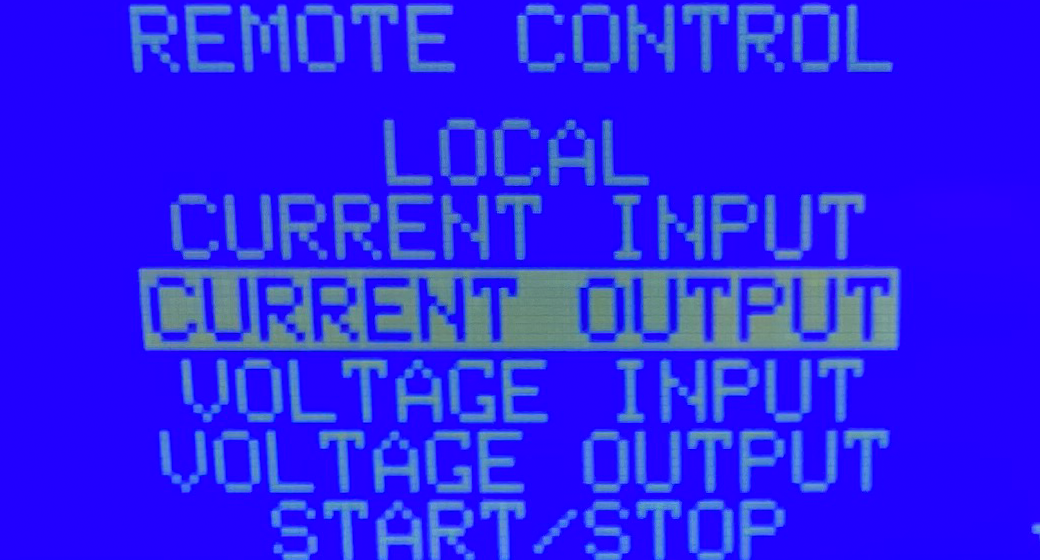
|
Note: Use the same maximum flow rate that you used in the Current Input step.
Speed Control Calibration
The Aqueduct Device Node outputs an analog signal to control the speed of the Masterflex L/S® pump. Prior to operation, a calibration routine should be performed to ensure accurate scaling of the output signal.
Caution: This calibration protocol will automatically set the pump to run while calibrating. Please take into consideration that the pump may cause fluid flow.
Calibration Procedure
- Navigate to the Sandbox in Lab Mode and select the Masterflex L/S® peristaltic pump that you wish to calibrate.
- Right-click the name of the of the Masterflex L/S® peristaltic pump device in the Device Menu or the Sandbox Icon. Click:
Actions > Calibrate
- Follow the on-screen prompts. The system will automatically set a low flow rate. The user must enter the flow rate displayed on the Masterflex L/S® pump screen and click "Set" to save the low point calibration. Press continue to perform the high point calibration.
- The system will then automatically set a higher flow rate. The user must enter the second flow rate displayed on the Masterflex L/S® pump screen and click "Set" to save the high point calibration.
- The system will then automatically stop the pump, and the new calibration factor will be stored on the Aqueduct Masterflex Device Node.
Note: The Device Node stores the calibration factor for one specific pump. The Masterflex L/S® pump and Aqueduct Device Node should be treated as a matched pair until re-calibration is completed.
Boxer 9QQ/15QQ
This page is under construction...
Pinch Valves
Aqueduct Pinch Valve
This page is under construction...
pH Probes
Aqueduct pH Electrode A/D
This page is under construction...
Pressure Transducers
Parker SciLog SciPres®
Table of Contents
- Device Specifications
- Connection and Setup
- SciLog SciPres® Configuration
- Integration with Aqueduct System
Device Specifications
| Feature | Value |
|---|---|
| Sensor Inputs | Up to three simultaneously |
| Sensor Readout | P1, P2 and P3; Differential pressure (dp); transmembrane pressure (TMP) |
For complete specifications, see Parker's documentation here.
Connection and Setup
Connect up to four SciLog SciPres® modules to the Aqueduct SciPres® Device Node with a straight-through, male-to-male DB-9 cable. Then, connect the SciPres® Device Node to an Aqueduct Hub using an Aqueduct CommCable.
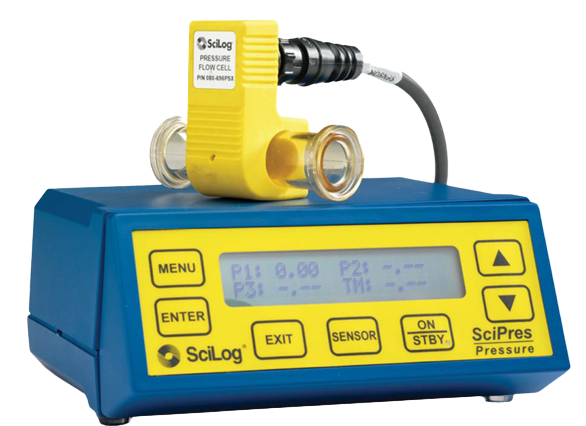
|
SciLog SciPres® Configuration
To properly interface with the Device Node, several configuration settings must be changed on the SciLog SciPres® module.
Main Menu
Use the touchscreen display to navigate to the Main Menu.
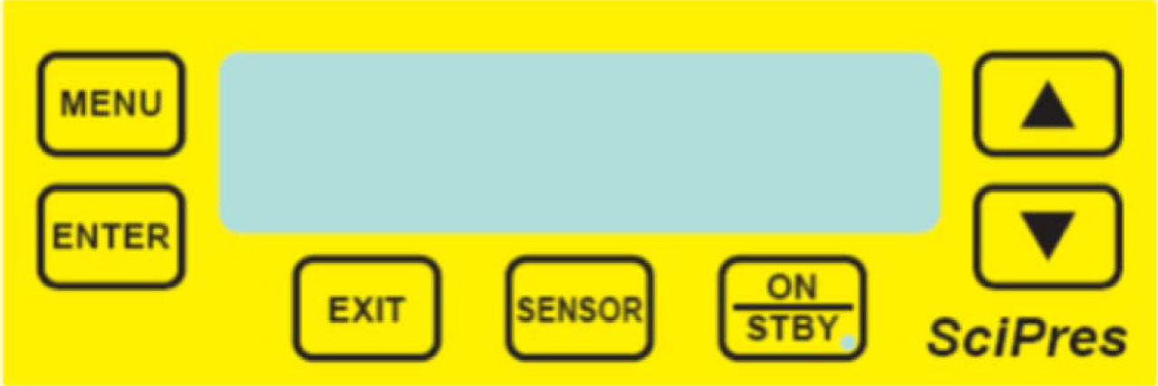
|
Communication Settings
Set the following communication settings on the SciLog SciPres® module:
- RS232 Protocol: BR: 9600, WL: 8, SB: 2, PT: N
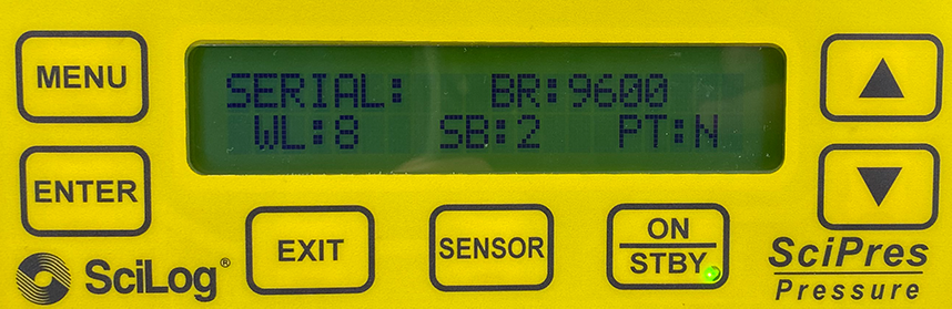
|
- Print Time: 1 SEC

|
Integration with Aqueduct System
Integrate your SciLog SciPres® modules into the Aqueduct system using the Aqueduct SciPres® Device Node.
The Aqueduct Device Node enables monitoring or recording of the pressure measured by up to three sensors simultaneously. The values can be used in Recipe scripts or for real-time monitoring and control.
Syringe Pumps
TriContinent C(X) Series
This page is under construction...
Harvard Apparatus
This page is under construction...
Applications
These pages contain a collection of real-world applications that utilize the capabilities of the Aqueduct system.
Each application consists of a complete package, including libraries, recipes, setups, layouts, and other resources that are tailored to the specific application's requirements. These applications serve as practical examples that demonstrate how the Aqueduct system can be applied in different contexts.
In addition to the software components, we include a real-world success story from each implementation. Photos of actual systems are included, showcasing the hardware setups and the integration with the Aqueduct system.
If you're interested in pursuing the implementation of one of these applications or would like to pursue a new application, please reach out to us at info@aqueductfluidics.com.
Filtration Application
The Filtration Application is a solution designed for automated tangential flow filtration processes. It offers:
-
Automated Control: The application provides automated control of the feed pump, permeate pump, and optional buffer pump.
-
Data Collection: Inline pressure transducers and balances are integrated into the system to enable real-time data collection. The application records the weight of buffer, feed, and permeate volumes, allowing for accurate monitoring and analysis of the filtration process.
-
Transmembrane Pressure Control: The application includes control algorithms that adjust the inline pinch valve to regulate the transmembrane pressure. The control algorithm can be modified based on the specific phase of the filtration process, ensuring optimal filtration conditions and improved performance.
-
Buffer Pump Control: To maintain a constant volume on the feed balance, the application provides control for the buffer pump rate. This control mechanism ensures consistent buffer solution levels, contributing to stable and efficient filtration operations.
-
Interactive Data Plotting and System Visualization: The Filtration Application offers interactive data plotting and system visualization tools.
-
Complete Logging: The application provides comprehensive logging capabilities, recording all relevant parameters and events throughout the filtration process.
pH Control Application
The pH Control Application utilizes peristaltic pumps and pH probes to automate pH control. It enables accurate and efficient regulation of pH in parallel reactions by adding a base. Key features of the pH Control Application include:
- Complete package with libraries, recipes, setups, layouts, and other resources tailored for pH control.
- Developed for the methacrylation of hyaluronic acid (HA) reaction, emphasizing precise pH regulation.
- Simulation capability to validate control algorithms and optimize performance.
- Two control algorithms: Smart Dose Addition (On/Off) and PID Control.
Dispensing and Formulation Application
The Dispensing and Formulation Application showcases control of syringe pumps in dispensing and formulation processes. Key features of this application include:
- Control of 12 syringe pumps operated in pairs or stations for versatile dispensing capabilities.
- Programming of dispense times and rates to vary the rate of reactant addition to the vessel over time.
- Support for various syringe sizes and pump types, including the actuation of a rotary valve for multiple input reagents.
- Dedicated waste output for syringe purging and an output to the reaction vessel.
- Ability to add timed delays in dispensing before or during the reaction.
- Calculation of cumulative volume dispensed for each station, with the option to plot it as a time series using an Aqueduct Recordable.
Tangential Flow Filtration
Table of Contents
- Tangential Flow Filtration
- Table of Contents
- Overview
- Success Story
- Control
- Hardware
- Try It Out
- Simulated Process Model Module
Overview
Tangential Flow Filtration (TFF) is a process used to separate or remove small solids from a feed liquid. A typical hardware setup for TFF consists of a:
-
Feed Pump: The feed pump is responsible for supplying the liquid feed to the TFF system. It provides the necessary pressure and flow rate to maintain the desired filtration conditions.
-
Tangential Flow Filter: The TFF filter is a key component that separates or removes small solids from the feed liquid. It consists of a membrane or porous material that allows the liquid to pass through while retaining the solids.
-
Permeate Pump: The permeate pump is used to collect the filtered liquid, known as permeate. It creates a pressure gradient that helps draw the permeate through the filter and into a collection container.
-
Buffer Pump: In some TFF setups, a buffer pump may be included in the hardware configuration. The buffer pump is responsible for supplying buffer solution or additional liquid to the TFF system. It helps maintain the desired volume and composition of the liquid within the system, ensuring optimal filtration conditions. The buffer pump can be controlled to adjust the flow rate and maintain a consistent buffer solution concentration throughout the process. Its integration enhances the control and stability of the TFF operation, especially when dealing with sensitive samples or complex filtration requirements.
-
Retentate Collector: The retentate collector receives the liquid that does not pass through the filter. It contains the retained solids or concentrated liquid and can be directed back to the feed tank for recirculation or further processing.
-
Flow Control Valves: Flow control valves, such as pinch valves or solenoid valves, are used to regulate the flow rates and control the direction of liquid within the TFF system.
-
Pressure Sensors: Pressure sensors are employed to monitor the pressure at different stages of the TFF system, including the feed, retentate, and permeate. These sensors provide real-time feedback on the system's performance and assist in controlling the filtration process.
-
Balance or Weighing System: In some TFF setups, a balance or weighing system may be included to measure the weight or mass of the liquid during the filtration process. This allows for precise monitoring and control of the filtration parameters, such as flow rates and mass accumulation.
Success Story
Background
A leading pharmaceutical company engaged Aqueduct to implement automation, control, and data logging to their TFF systems. The project aimed to provide user controls and capture process parameters to ensure consistency from operator to operator, enhancing efficiency and reproducibility in their operations.
Challenges
- Ensuring precise control and monitoring of pressures throughout the TFF process
- Integrating multiple hardware components into the system
- Validating and optimizing the process prior to physical implementation to minimize risks and costs
- Documentation and knowledge transfer to ensure long-term operability and maintenance of the system
Key Features:
-
Simulation-Based Process Refinement:
- Utilized the Aqueduct platform's simulated model to estimate pressures and monitor balance volume accumulation during the TFF process.
- Iteratively refined and optimized the process logic exclusively in the simulation mode, ensuring an understanding of the system's behavior and performance.
-
Hardware Integration:
- Integrated three Masterflex Peristaltic Pumps, an Aqueduct-designed pinch valve, three Ohaus Scout and Adventurer balances, and three Parker Scilog pressure transducers into the TFF system.
- Ensured communication between the hardware components and the Aqueduct platform for control, accurate measurements, and real-time feedback.
-
Initial Concentration, Diafiltration, and Ultrafiltration:
- Leveraged the Aqueduct platform's capabilities to perform initial concentration, diafiltration, and ultrafiltration steps within the TFF process.
- Ensured precise control and accurate monitoring of the concentration and volume exchange processes.
-
Centralized Data Logging:
- Building on top of the Aqueduct platform, implemented a central data logging platform to capture real time data from multiple systems and store process parameters in a centralized database.
Simulated Process Model Module
As part of the development process, Aqueduct implemented a process model to simulate inline pressures as a function of pump rates, pinch valve position, and filter parameters. Using the model, control logic for the pinch valve was refined and validated before running the process with real hardware. You can see the details of the pressure model here.
Additionally, the simulated process includes an optional error factor for the volume collection rate on the feed balance and the setpoint rate for the buffer pump. This error simulates tubing wear and was used to implement weight-driven control of the buffer pump instead of relying on the nominal setpoint to maintain a constant feed vessel weight.
Control
The TFF simulated model in the Aqueduct platform allowed for testing control algorithms for the TFF processes prior to applying them in the laboratory with real reagents and equipment.
Key control points for the TFF system include:
-
Feed Pump Rate: The TFF process model incorporates feed pump rate adjustment logic to ensure optimal performance. This logic dynamically adjusts the buffer pump rate based on the deviation between the actual weight accumulation on the balance and the target flow rate of the feed pump.
-
PID Control of Pinch Valve: The Aqueduct platform supports PID (Proportional-Integral-Derivative) control of the pinch valve to regulate the transmembrane pressure in the TFF system.
-
Target Permeate Collection Weight: The process also allows you to set a target permeate collection weight. By specifying the desired weight, the system can automatically adjust the TFF process parameters to achieve the desired volume of permeate collected.
Adjusting Feed Pump Rate
The TFF process model incorporates a feed pump rate adjustment logic to ensure optimal performance. This feature helps account for factors such as tubing wear and pump deviations from the setpoint, ensuring accurate measurements and precise control in the TFF process.
The adjustment logic focuses on monitoring the deviation between the actual weight accumulation on the balance and the target flow rate of the feed pump. By continuously comparing the accumulation rates of the scales with set thresholds, the model can make necessary adjustments to the feed pump rate.
The adjustment algorithm operates in two modes:
-
Mode 1: Δm/Δt Adjustment
- In this mode, the buffer pump rate is adjusted to force the rate of change (Δm/Δt) on the feed balance to zero. This helps maintain a stable product concentration and minimize fluctuations caused by variations in the feed pump rate.
-
Mode 2: Setpoint-driven Adjustment
- In this mode, the buffer pump rate is adjusted to drive the feed balance mass to a specific setpoint at a specified rate. This ensures that the weight accumulation on the balance aligns with the desired setpoint, enabling accurate control of the TFF process.
The adjustment algorithm takes into account parameters such as maximum deviation thresholds, maximum pump adjustment limits, and target mass or time to reach the setpoint. By dynamically modifying the pump rates within the specified limits, the model compensates for tubing wear, pump deviations, and other factors that may affect the balance readings.
While the feed pump adjustment logic is specifically designed for the real application of the TFF process, it is important to note that the logic can be tested and validated in the simulation mode. By configuring the simulated balance instrument to deviate from the pump's target flow rate, the model's performance can be assessed and fine-tuned to ensure accurate measurements and precise control.
Hardware
The delivered TFF system was comprised of two enclosures.
The Main Enclosure (pictured right) serves as the central hub of the TFF System. It houses a computer that runs the Aqueduct software application and is equipped with 5 Device Nodes. These Device Nodes provide the interface for connecting and controlling the various components. In the default configuration, the Device Nodes facilitate communication with 3 Masterflex L/S Peristaltic Pumps, 3 Ohaus Adventurer balances, and 3 Parker SciLog pressure transducers. However, we can incorporate different models or brands of pumps, pressure transducers, or balances as needed.
The Pinch Valve Enclosure (pictured left) accommodates a Pinch Valve and the necessary driver electronics. It can be positioned close to the process and is connected to the Main Enclosure with a dedicated power and communications cable.
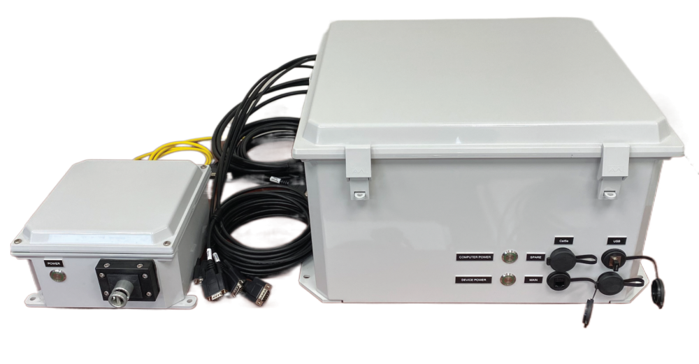
|
Try It Out
To run the TFF recipe locally in simulation mode:
-
Install the Aqueduct application.
-
Download the Aqueduct examples repository and extract the compressed archive.
-
Navigate to the Library page and upload the
/apps/filtration/tffdirectory from the extracted archive. -
Navigate to the Dashboard page and upload the necessary .recipe, .setup, and .layout files found in the
/apps/filtration/modelsdirectory. -
Activate the
TFF - Full operationrecipe from your Dashboard and navigate to the Sandbox to view the simulated process.
Pressure Model
Pressure Calculation and Assumptions
The PressureModel class in the provided Python code is responsible for estimating and updating the pressures involved in Tangential Flow Filtration (TFF) based on the current pump flow rates and pinch valve position. This section explains the calculation and assumptions made in the pressure modeling process.
Pressure Estimation
The class includes several methods to calculate the pressures at different stages of the TFF process, namely P1 (feed pressure), P2 (retentate pressure), and P3 (permeate pressure). These calculations consider the flow rates, pinch valve position, and pressure drops between different sections of the TFF system.
calc_delta_p_feed_retentate(R1)
This method calculates the pressure drop between the feed and retentate using the flow rate (R1) in the pass-through leg of the TFF filter. The calculation assumes a relationship where the pressure drop is inversely proportional to the square of the Cv value of the retentate leg of the TFF filter.
The equation is given by:
ΔP_feed_retentate = 1 / ((Cv * 0.865 / R1)^2)
where ΔP_feed_retentate is the pressure drop between feed and retentate, Cv is the Cv value of the retentate leg of the TFF filter.
calc_pv_cv(PV)
This method calculates the Cv (flow coefficient) of the pinch valve based on its position (PV). The calculation uses a non-linear expression that decreases as the pinch valve position increases, following a relationship of (percent open)^-2 with an onset position of 0.3 (30%).
The equation is given by:
Cv =
    if PV < 0.3 {
        100 - (1 / (PV^2))
    } else {
        100
    }
where Cv is the Cv of the pinch valve, and PV is the pinch valve position.
calc_delta_p_retentate(R1, PV)
This method calculates the pressure drop between the retentate and permeate based on the flow rate (R1) and pinch valve position (PV). The calculation assumes a relationship similar to calc_delta_p_feed_retentate(), where the pressure drop is inversely proportional to the square of the Cv value obtained from calc_pv_cv().
The equation is given by:
ΔP_retentate_permeate = 1 / ((Cv * 0.865 / R1)^2)
where ΔP_retentate_permeate is the pressure drop between retentate and permeate, Cv is the Cv of the pinch valve obtained from calc_pv_cv(), and R1 is the flow rate in the pass-through leg of the TFF filter.
calc_p1(R1, PV, P2)
This method calculates the P1 pressure based on the flow rate (R1), pinch valve position (PV), and the P2 pressure. The calculation adds the pressure drop obtained from calc_delta_p_retentate() to the P2 pressure.
The equation is given by:
P1 = P2 + ΔP_retentate_permeate
where P1 is the feed pressure, P2 is the retentate pressure, and ΔP_retentate_permeate is the pressure drop between retentate and permeate.
Pressure Update
The calc_pressures() method is responsible for updating the pressures in the TFF system using the model equations. It calls the aforementioned methods to calculate P1, P2, and P3 based on the available data (flow rates, pinch valve position) and limits the pressures to a maximum value of 50.
The updated pressures are then set as simulated values for the corresponding devices in the Aqueduct system, ensuring that the simulated TFF process reflects the calculated pressures.
It's important to note that the provided code represents a simplified model for estimating the pressures in the TFF process. The calculations and assumptions made in the model may not capture all the intricacies of the real TFF system and should be further refined and validated based on the specific requirements and characteristics of the actual TFF process.
pH Control
Introduction
Controlling pH is crucial in many laboratory workflows as numerous reactions are sensitive to pH changes. This pH Control & Monitoring Library provides a comprehensive solution for implementing pH control in reactions using peristaltic pumps and pH probes. The library was originally developed for the methacrylation of hyaluronic acid (HA), a specific reaction where the pH needs to be precisely regulated to drive the reaction forward. During the methacrylation of HA, methacrylic anhydride (MA) is added to an aqueous HA solution, causing a decrease in pH. To maintain the optimal pH level, a base, usually NaOH, needs to be continuously added as the reaction progresses.
For more information on the reaction and applications of hyaluronic acid, please refer to the following references:
The kinetics of the reaction evolve with time, necessitating a higher rate of NaOH addition during the initial stages of the reaction.
Control
Smart Dose Addition (On/Off)
The Smart Dose Addition algorithm adds base to the reaction vessel in finite doses when the pH drops below the setpoint value. To calculate the dose volume, the algorithm takes into account the effect of the previous dose (change in pH per added volume) and adjusts the next dose volume to reach the desired setpoint. The algorithm includes a limit on the maximum change in dose volume for consecutive doses.
PID
The PID Control algorithm continuously adds base to the reaction vessel to achieve the target pH setpoint. The rate of base addition is calculated by the PID controller, which constantly evaluates the error (setpoint - current pH value), cumulative error (sum of errors), and rate of change of the error (d_error/dt). The PID controller adjusts the base addition rate based on these parameters to maintain the pH at the desired setpoint.
Hardware
The delivered system included 3 Boxer 9QQ peristaltic pumps and 3 pH electrode analog-to-digital converters. The pumps were mounted on a vertical scaffold to allow them to be positioned close to the reaction flasks inside a fume hood.
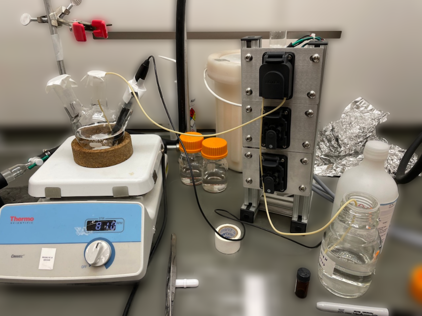
The pump chassis allows the 3 peristaltic pumps to be located inside a fume hood close to the reaction flask.
|
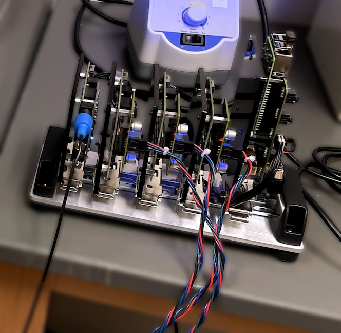
The electronics chassis located outside of the fume hood.
|
Try It Out
To run the pH control recipe locally in simulation mode:
-
Install the Aqueduct application.
-
Download the Aqueduct examples repository and extract the compressed archive.
-
Navigate to the Library page and upload the
/apps/ph_control/ph_controldirectory from the extracted archive. -
Navigate to the Dashboard page and upload the necessary .recipe, .setup, and .layout files found in the
/apps/ph_control/modelsdirectory. -
Activate the
pH - PID controlrecipe from your Dashboard and navigate to the Sandbox to view the simulated process.
Modeling the Reaction
The Aqueduct platform provides the ability to simulate the reaction process before running it with real reagents and equipment. This simulation capability is beneficial for validating control algorithms and optimizing their performance.
Constant Rate Kinetic Decay (Smart Dose)
In the Smart Dose control algorithm, the decay in pH rate-of-change over time is modeled using a linear expression. Initially, the rate of pH decrease (dpH/dt) is large and negative. As the reaction progresses, the rate of pH change becomes smaller but remains negative. This behavior can be described by the following expression:
dpH_dt(t) = ROC_start + (t_now - t_start) * delta_ROC_dt
Where:
-
dpH_dt: Rate of change in pH as a function of time. -
ROC_start: Rate of change in pH at the start of the reaction (t_start). -
t_now: Current time. -
t_start: Reaction start time. -
delta_ROC_dt: Decay in reaction kinetics over time.
The ReactionModel class in the models.py file encapsulates this behavior.
Base Addition Rate Dependent (PID)
The PID control algorithm models the pH rate-of-change as a function of the base addition rate. As the reaction progresses, the sensitivity of pH rate-of-change to the base addition rate increases. The behavior can be described by the following expression:
dpH_dt(t, base_addition_rate) = ROC_offset + (ROC_init + (t_now - t_start) * delta_ROC_dt) * base_addition_rate
Where:
dpH_dt: Rate of change in pH as a function of time and base addition rate.ROC_offset: Intrinsic rate of change in pH due to the reaction.ROC_init: Rate of change in pH at the start of the reaction (t_start).t_now: Current time.t_start: Reaction start time.delta_ROC_dt: Decay in reaction kinetics over time.base_addition_rate: Rate of base addition in mL/min.
The PidModel class in the models.py file encapsulates this behavior.
Dispensing & Formulation
Background
A leading specialty chemical company engaged Aqueduct to implement programmable control of 12 syringe pumps for timed dispensing in a synthesis screening study. The implementation including full priming, purging, and reloading logic to allow for syringes of various sizes to be used to target different dispense rate ranges.
Key Features:
-
Simulation-Based Process Refinement:
- Calculation of cumulative volume dispensed for each station, with the option to plot it as a time series using an Aqueduct Recordable.
-
Hardware Integration:
- Control of 12 TriContinent C-Series syringe pumps using the CanBus interface.
Hardware
The delivered Dispensing system was comprised of a control enclosure with a custom circuit board and cable harness to allow for daisy chaining 12 pumps.
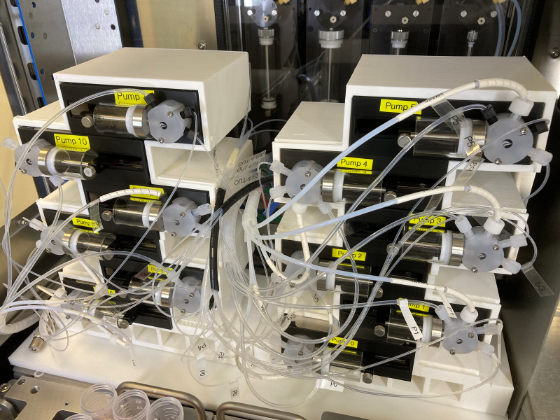
|
Try It Out
To run the dispensing recipe locally in simulation mode:
-
Install the Aqueduct application.
-
Download the Aqueduct examples repository and extract the compressed archive.
-
Navigate to the Library page and upload the
/apps/dispensing/dispensingdirectory from the extracted archive. -
Navigate to the Dashboard page and upload the necessary .recipe, .setup, and .layout files found in the
/apps/dispensing/modelsdirectory. -
Activate the
CoDispenserecipe from your Dashboard and navigate to the Sandbox to view the simulated process.
FAQ
- Libraries, Recipes, Setups, and Layouts
- Sim Mode and Lab Mode
- Tabs, Tab Containers, and Widgets
- Menus & Icons
- Recipe Lifecycle
Libraries, Recipes, Setups, and Layouts
-
Q: What is a Library?
A: A Library is a collection of related Python classes and methods. Libraries are intended to allow for reuse of common functionality across multiple Recipes.
-
Q: How do I upload or delete a Library?
A: Use the Library page on the Dashboard to upload or delete a Library. See complete instructions here.
-
Q: What is a Recipe Script?
A: A Recipe Script is simply a Python file (
.py) that is run in the Aqueduct environment. It contains the logic to execute your process. A Recipe Script can import from one or more local Libraries and the standard Python library. -
Q: What is a Recipe file?
A: A Recipe file (
.recipeextension) contains a Recipe Script, a Setup, and (optionally) a Layout. It contains all of the data necessary to recreate a user interface (Device, Container, and Connection icon arrangement and Widget layout and metadata) and the logic (contained in the Recipe Script) to execute a protocol or processs. -
Q: What is a Setup file?
A: A Setup file (
.setupextension) contains the type and number of:- Devices: pumps, valves, sensors, or other hardware that has I/O
- Containers: beakers, vials, or other 'passive' labware
- Connections: representations of tubing, both external and internal to Devices or Containers
A Setup also contains the position and orientation data of the icons used to generate the user interface.
-
Q: What is a Layout file?
A: A Layout file (
.layoutextension) contains the Widget metadata that generates the user interface. For instance, the specific data series plotted on a Chart Widget on Tab 1 is stored in a Layout file. You can tailor the Layout arrangement to your preferences and save the configuration as a Layout file for reuse later.
Sim Mode and Lab Mode
-
Q: What is Simulation Mode?
A: Simulation Mode is a feature in the Aqueduct application that allows users to simulate Recipes without physical hardware. It enables testing and validation of Recipes using virtual devices and containers.
-
Q: What is Lab Mode?
A: Lab Mode is the operational mode of the Aqueduct application where Recipes are executed using real hardware devices and containers in a laboratory setting. It allows for performing actual experiments and processes in a controlled environment.
Tabs, Tab Containers, and Widgets
-
Q: What is a Tab?
A: A Tab is a workspace within the Aqueduct application where you can organize and group Tab Containers and Widgets. Each Tab provides a separate area for adding Tab Containers and Widgets.
-
Q: What is a Tab Container?
A: A Tab Container is a container within a Tab that holds and organizes one or more Widgets. It acts as a layout container, allowing you to arrange Widgets within a Tab according to your preferences. You can have multiple Tab Containers within a single Tab.
-
Q: What is a Widget?
A: A Widget represents a functional component or visual element in the Aqueduct user interface. Widgets can display data, receive input, or perform specific actions. Examples of Widgets include charts, tables, buttons, input fields, and displays for sensor readings.
-
Q: How do I add a Tab?
A: To add a Tab to the workspace, click the plus icon located to the right of the left sidebar menu. This will create an empty Tab where you can organize and design your interface.
-
Q: How do I add a Tab Container?
A: To add a Tab Container within a Tab, click the plus icon on the vertical Tab Container menu at the right side of the screen. This will create an empty Tab Container where you can place and organize your Widgets.
-
Q: How do I add a Widget to a Tab Container?
A: To add a Widget to a Tab Container, click the plus icon on the vertical Tab Container menu. This will open a menu where you can select the type of Widget you want to add. Choose the desired Widget, and it will be added to the Tab Container.
-
Q: What is a Sandbox Widget?
A: A Sandbox Widget is a type of Widget that provides a blank canvas for experimentation and testing. It allows you to interact with various features and functionalities of the Aqueduct application without the need for specific data or devices. It is a versatile Widget that can be customized to suit your needs.
Menus & Icons
Left Sidebar Menu Icons
The Left Sidebar Menu provides:
- access to Setup and Setpoint controls
- Recipe status visualization and execution control
- access to the Settings menu
|
||||||||||||||||||||||||||||||||||||||||||


Recipe Status Indicators
|
|||||||||||||||||||||||||||||||||


The Recipe Lifecycle
Recipes progress through a lifecycle of steps as they are executed in the Aqueduct environment. Knowledge of this lifecycle and the transitions between steps is crucial for understanding how the system will respond to Recipe control inputs.
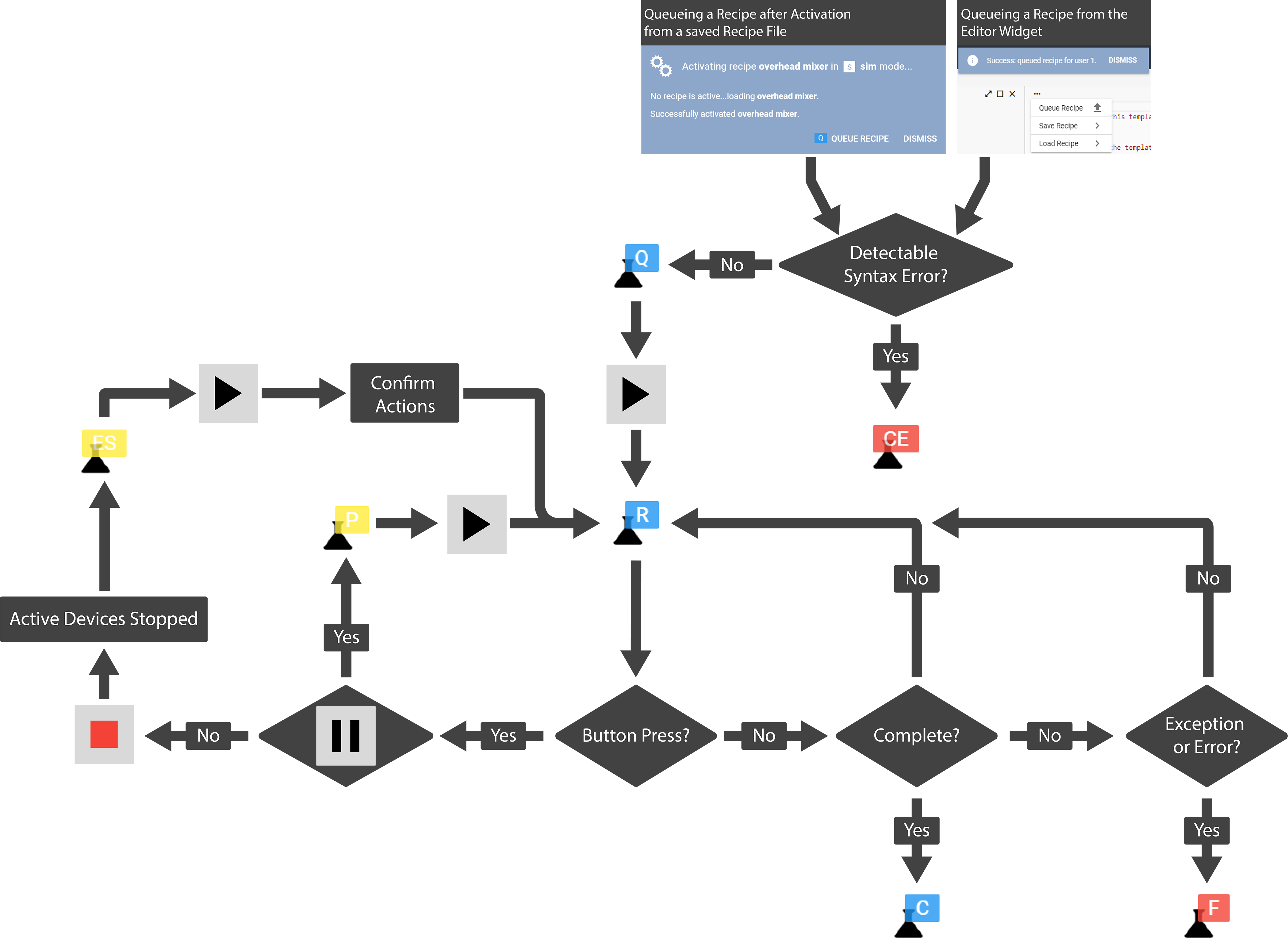
Queued

|
A Recipe begins its lifecycle in the Queued state. Recipes may be queued directly from the Editor Widget menu in the Sandbox interface (as shown in Use the API) or by clicking the Queue Recipe button after activating a saved Recipe file.
If another Recipe is active - Running, Paused, or E-Stopped - you'll receive a warning before queueing proceeds.
When a recipe is queued, the code that you've saved in a Recipe or generated in the editor is executed in a Python interpreter. At this stage, the execution is paused if the pause_on_queue setting is enabled. The pause_on_queue setting determines whether a recipe should be paused after queuing. It is achieved by passing the proper arguments to the Python process on spawn.
You can configure the pause_on_queue setting in the Aqueduct application. By default, if the setting is not specified, it is set to true. When a recipe is paused after queuing, it is considered ready to be executed. You can identify a queued recipe by the blue Q badge displayed in the Recipe Status indicator.
Please note that the behavior of the pause_on_queue setting can be customized based on your specific requirements.
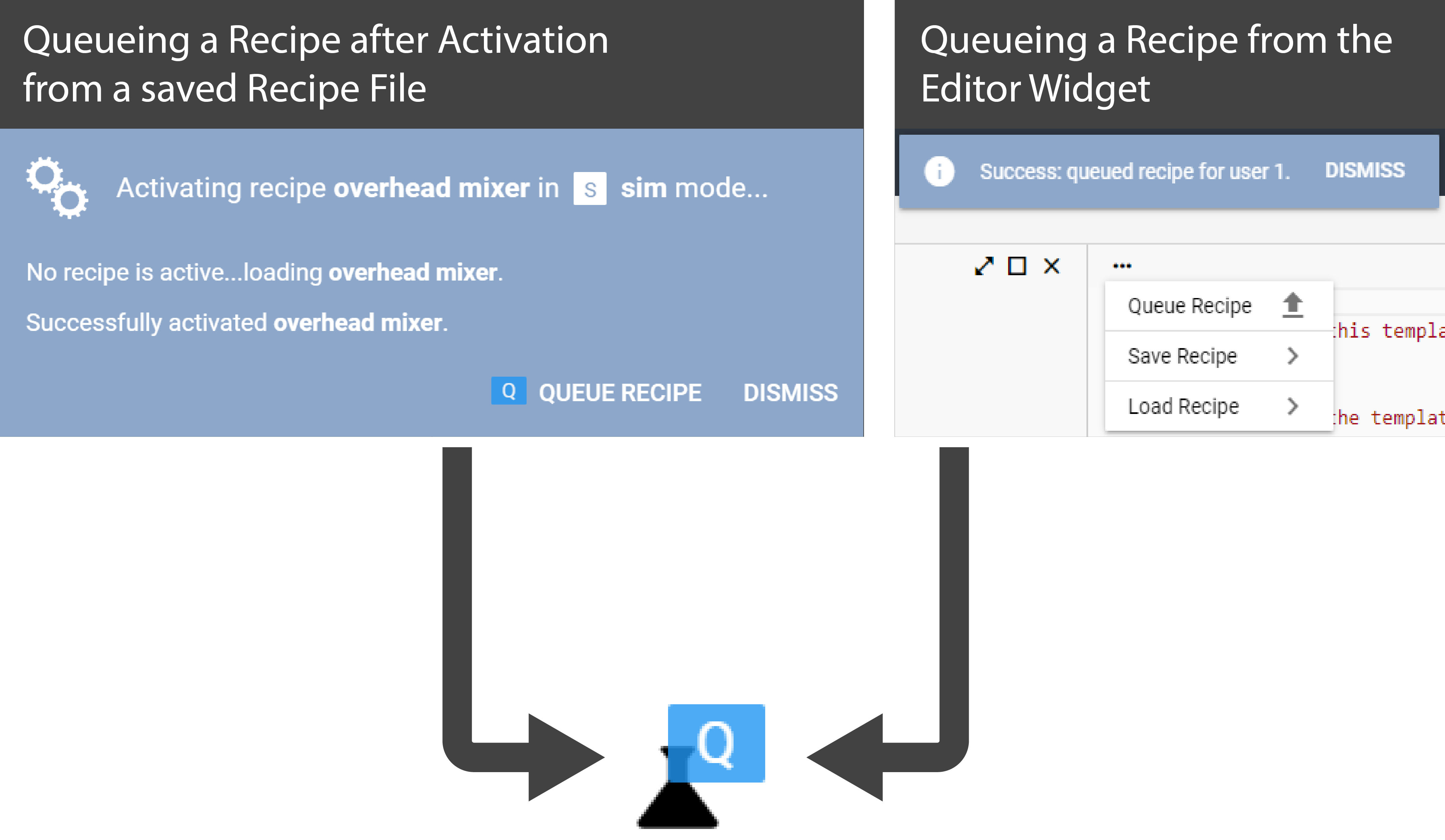
Running

|
The Running state indicates that your Recipe's Python process is active and executing.
There are three possible ways to enter the Running state:
-
After a Recipe has been Queued, you can begin execution by pressing the Start/Resume Recipe Button in the left sidebar menu. The Recipe transitions into the Running state.
-
After a Recipe has been Paused, you can resume execution by pressing the Start/Resume Recipe Button in the left sidebar menu. The Recipe transitions into the Running state without any further input needed from the user.
-
After a Recipe has been E-Stopped, you can resume execution by pressing the Start/Resume Recipe Button in the left sidebar menu. Prior to restarting the Recipe process, the user must confirm which Device actions to execute before resuming. The available Device actions are determined from the state of the Device when the Recipe was E-Stopped.
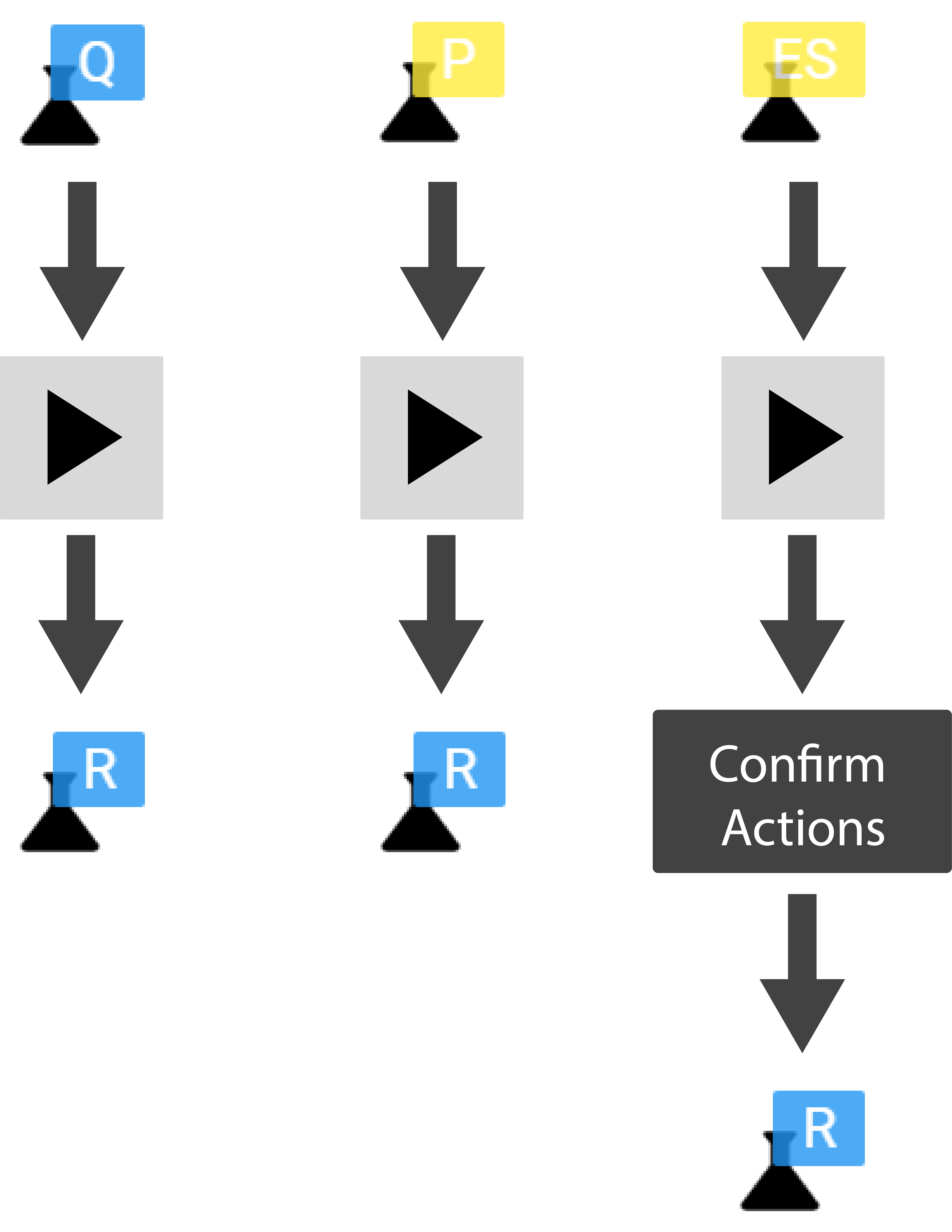
Paused

|
The Paused state indicates that your Recipe's Python process is active but has been temporarily paused to prevent further execution.
The paused state may be entered from the running state by pressing the Pause Recipe Button in the left sidebar menu. The Recipe transitions into the Paused state without any further input needed from the user.
In contrast to an E-Stop action, no Device actions are executed when a Recipe is paused. The Devices are left in the same state they were in before the pause button was pressed. For instance, if an MFPP Peristaltic Pump device was operating at 20 mL/min before the pause button was pressed, the pump will continue to operate after the button has been pressed.

While a Recipe is Paused, a user may still interact with and control any Devices by using their control buttons.
E-Stopped

|
The E-Stopped state indicates that your Recipe's Python process is active but has been temporarily paused to prevent further execution.
The E-Stopped state may be entered from the running state by pressing the E-Stop Recipe Button in the left sidebar menu. The Recipe transitions into the E-Stopped state without any further input needed from the user.
All Devices that are considered active when the E-Stop button is pressed, such as operating pumps or robotic arms, are issued commands to stop any motion. Passive devices, such as balances, pH probes, or other sensors that simply transmit data and do not move, are left unaffected.
While a Recipe is E-Stopped, a user may still interact with and control any Devices using their control buttons.
Failed

|
The Failed state indicates that your Python process has encountered an exception or error and exited. A Recipe cannot be resumed or restarted after it has failed.
When a Recipe fails, the source of the error is captured by the application. You can view information about the error by pressing the Recipe Status Indicator in the left sidebar menu and selecting:
> Show Error
A Recipe Error Widget will be added to your window that contains the traceback of the error source.
Killed

|
The Killed state indicates that your Python process has been terminated permanently. A Recipe cannot be resumed or restarted after it has been Killed.
To kill an active Recipe, press the Recipe Status Indicator in the left sidebar menu and select:
> Kill Recipe > Confirm
No Device commands are issued when the Recipe is killed.
Contact us at info@aqueductfluidics.com.
![]()